in terms of Whittaker functions

SearchAdvancedHelp

(0.011 seconds)

11—20 of 38 matching pages

11: 13.28 Physical Applications

§13.28 Physical Applications

… ►and $V_{\kappa ,\mu }^{(j)}(z)$, $j=1,2$, denotes any pair of solutions of Whittaker’s equation (13.14.1). … ►For potentials in quantum mechanics that are solvable in terms of confluent hypergeometric functions see Negro et al. (2000). ►

§13.28(ii) Coulomb Functions

…

12: Bibliography O

… ►

Whittaker functions with both parameters large: Uniform approximations in terms of parabolic cylinder functions. Proc. Roy. Soc. Edinburgh Sect. A 86 (3-4), pp. 213–234.

ⓘ

External Links:

ISSN 0308-2105, MathReview (P. F. Hsieh), ZentralBlatt

Referenced by:

§13.20(iii), §13.20(iv).

Encodings:

BibTeX

…

13: 13.21 Uniform Asymptotic Approximations for Large $\kappa$

… ►For a uniform asymptotic expansion in terms of Airy functions for $W_{\kappa ,\mu }\left(4\kappa x\right)$ when $\kappa$ is large and positive, $\mu$ is real with $|\mu |$ bounded, and $x\in [\delta ,\mathrm{\infty })$ see Olver (1997b, Chapter 11, Ex. 7.3). …

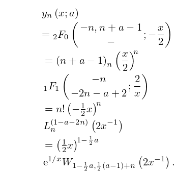
14: 18.34 Bessel Polynomials

… ►

18.34.1 $$y_n(x;a)={}_2{}^{}F_0^{}(\genfrac{}{}{0pt}{}{-n,n+a-1}{-};-\frac{x}{2})={\left(n+a-1\right)}_n{\left(\frac{x}{2}\right)}^n{}_1{}^{}F_1^{}(\genfrac{}{}{0pt}{}{-n}{-2n-a+2};\frac{2}{x})=n!{\left(-\frac{1}{2}x\right)}^n{L}_n^{(1-a-2n)}\left(2x^{-1}\right)={\left(\frac{1}{2}x\right)}^{1-\frac{1}{2}a}{\mathrm{e}}^{1/x}{W}_{1-\frac{1}{2}a,\frac{1}{2}(a-1)+n}\left(2x^{-1}\right).$$

ⓘ

Defines:

$y_n(x;a)$: Bessel polynomial

Symbols:

${}_p{}^{}F_q^{}(a_1,\mathrm{\dots },a_p;b_1,\mathrm{\dots },b_q;z)$ or ${}_p{}^{}F_q^{}(\genfrac{}{}{0pt}{}{a_1,\mathrm{\dots },a_p}{b_1,\mathrm{\dots },b_q};z)$: alternatively ${}_p{}^{}F_q^{}(𝐚;𝐛;z)$ or ${}_p{}^{}F_q^{}(\genfrac{}{}{0pt}{}{𝐚}{𝐛};z)$
generalized hypergeometric function, ${}_1{}^{}F_1^{}(a;b;z)$: $=M(a,b,z)$ notation for the Kummer confluent hypergeometric function, $L_n^{(\alpha )}\left(x\right)$: Laguerre (or generalized Laguerre) polynomial, ${\left(a\right)}_n$: Pochhammer’s symbol (or shifted factorial), $W_{\kappa ,\mu }\left(z\right)$: Whittaker confluent hypergeometric function, $\mathrm{e}$: base of natural logarithm, $!$: factorial (as in $n!$), $n$: nonnegative integer and $x$: real variable

Proved:

Grosswald (1978, p.38, Theorem 1); Combine (18.5.12) and items (i), (v), (vii) of the mentioned theorem for $b=2$(proved)

Referenced by:

(18.34.2), (18.34.7_1), §18.34(i), §18.34(i), Erratum (V1.2.0) for Equation (18.34.1)

Permalink:

http://dlmf.nist.gov/18.34.E1

Encodings:

pMML, png, TeX

Addition (effective with 1.2.0):

This equation was updated to include the definition of Bessel polynomials interms of Laguerre polynomials and the Whittaker confluent hypergeometric function.

See also:

Annotations for §18.34(i), §18.34 and Ch.18

… ►expressed in terms of Romanovski–Bessel polynomials, Laguerre polynomials or Whittaker functions, we have …

15: 13.20 Uniform Asymptotic Approximations for Large $\mu$

… ►

§13.20(i) Large $\mu$, Fixed $\kappa$

… ► ►It should be noted that (13.20.11), (13.20.16), and (13.20.18) differ only in the common error terms. … ►These approximations are in terms of Airy functions. … ►

16: 33.16 Connection Formulas

… ►

§33.16(iii) $f$ and $h$ in Terms of $W_{\kappa ,\mu }\left(z\right)$ when

… ►

§33.16(v) $s$ and $c$ in Terms of $W_{\kappa ,\mu }\left(z\right)$ when

…

17: Errata

… ►

18.34.1 $$y_n(x;a)={}_2{}^{}F_0^{}(\genfrac{}{}{0pt}{}{-n,n+a-1}{-};-\frac{x}{2})={\left(n+a-1\right)}_n{\left(\frac{x}{2}\right)}^n{}_1{}^{}F_1^{}(\genfrac{}{}{0pt}{}{-n}{-2n-a+2};\frac{2}{x})=n!{\left(-\frac{1}{2}x\right)}^n{L}_n^{(1-a-2n)}\left(2x^{-1}\right)={\left(\frac{1}{2}x\right)}^{1-\frac{1}{2}a}{\mathrm{e}}^{1/x}{W}_{1-\frac{1}{2}a,\frac{1}{2}(a-1)+n}\left(2x^{-1}\right)$$

This equation was updated to include the definition of Bessel polynomials in terms of Laguerre polynomials and the Whittaker confluent hypergeometric function.

… ►

A sentence was added in §8.18(ii) to refer to Nemes and Olde Daalhuis (2016). Originally §8.11(iii) was applicable for real variables $a$ and $x=\lambda a$. It has been extended to allow for complex variables $a$ and $z=\lambda a$ (and we have replaced $x$ with $z$ in the subsection heading and in Equations (8.11.6) and (8.11.7)). Also, we have added two paragraphs after (8.11.9) to replace the original paragraph that appeared there. Furthermore, the interval of validity of (8.11.6) was increased from to the sector , and the interval of validity of (8.11.7) was increased from $\lambda >1$ to the sector $\lambda >1$, $|\mathrm{ph}a|\le \frac{3\pi }{2}-\delta$. A paragraph with reference to Nemes (2016) has been added in §8.11(v), and the sector of validity for (8.11.12) was increased from $|\mathrm{ph}z|\le \pi -\delta$ to $|\mathrm{ph}z|\le 2\pi -\delta$. Two new Subsections 13.6(vii), 13.18(vi), both entitled Coulomb Functions, were added to note the relationship of the Kummer and Whittaker functions to various forms of the Coulomb functions. A sentence was added in both §13.10(vi) and §13.23(v) noting that certain generalized orthogonality can be expressed in terms of Kummer functions.

…

18: 22.14 Integrals

… ►With $x\in ℝ$, … ►For alternative, and symmetric, formulations of the results in this subsection see Carlson (2006a). … ►The indefinite integral of a 4th power can be expressed as a complete elliptic integral, a polynomial in Jacobian functions, and the integration variable. … ►For indefinite integrals of squares and products of even powers of Jacobian functions in terms of symmetric elliptic integrals, see Carlson (2006b). … ► …

19: 5.11 Asymptotic Expansions

… ►The expansion (5.11.1) is called Stirling’s series (Whittaker and Watson (1927, §12.33)), whereas the expansion (5.11.3), or sometimes just its leading term, is known as Stirling’s formula (Abramowitz and Stegun (1964, §6.1), Olver (1997b, p. 88)). … ►If the sums in the expansions (5.11.1) and (5.11.2) are terminated at $k=n-1$ ($k\ge 0$) and $z$ is real and positive, then the remainder terms are bounded in magnitude by the first neglected terms and have the same sign. … ►For the remainder term in (5.11.3) write … ►For re-expansions of the remainder terms in (5.11.1) and (5.11.3) in series of incomplete gamma functions with exponential improvement (§2.11(iii)) in the asymptotic expansions, see Berry (1991), Boyd (1994), and Paris and Kaminski (2001, §6.4). … ►For the error term in (5.11.19) in the case $z=x(>0)$ and $c=1$, see Olver (1995). …

20: 20.4 Values at $z$ = 0

§20.4 Values at $z$ = 0

►

§20.4(i) Functions and First Derivatives

… ►

20.4.2 $${\theta }_1^{\prime }(0,q)=2q^{1/4}\prod _{n=1}^{\mathrm{\infty }}{\left(1-q^{2n}\right)}^3=2q^{1/4}{(q^2;q^2)}_{\mathrm{\infty }}^3,$$

ⓘ

Symbols:

${\theta }_j(z,q)$: theta function, ${(a;q)}_n$: $q$-Pochhammer symbol (or $q$-shifted factorial), $n$: integer and $q$: nome

Referenced by:

Erratum (V1.0.28) for Equation (20.4.2)

Permalink:

http://dlmf.nist.gov/20.4.E2

Encodings:

pMML, png, TeX

Addition (effective with 1.0.28):

The representation interms of ${(q^2;q^2)}_{\mathrm{\infty }}^3$ was added to this equation.

See also:

Annotations for §20.4(i), §20.4 and Ch.20

►

20.4.3 $${\theta }_2(0,q)=2q^{1/4}\prod _{n=1}^{\mathrm{\infty }}\left(1-q^{2n}\right){\left(1+q^{2n}\right)}^2,$$

ⓘ

Symbols:

${\theta }_j(z,q)$: theta function, $n$: integer and $q$: nome

Referenced by:

(20.10.3)

Permalink:

http://dlmf.nist.gov/20.4.E3

Encodings:

pMML, png, TeX

See also:

Annotations for §20.4(i), §20.4 and Ch.20

… ►

Jacobi’s Identity

…