imaginary-modulus%20transformations

♦ 1—10 of 279 matching pages ♦

(0.005 seconds)

1—10 of 279 matching pages

1: 1.14 Integral Transforms

§1.14 Integral Transforms

►

§1.14(i) Fourier Transform

… ►

§1.14(iii) Laplace Transform

… ►

Fourier Transform

… ►

Laplace Transform

…

2: 15.19 Methods of Computation

… ►For

z\in\mathbb{C}

it is possible to use the linear transformations in such a way that the new arguments lie within the unit circle, except when

z={\mathrm{e}}^{\pm\pi\mathrm{i}/3}

. This is because the linear transformations map the pair

\{{\mathrm{e}}^{\pi\mathrm{i}/3},{\mathrm{e}}^{-\pi\mathrm{i}/3}\}

onto itself. However, by appropriate choice of the constant

z_{0}

in (15.15.1) we can obtain an infinite series that converges on a disk containing

z={\mathrm{e}}^{\pm\pi\mathrm{i}/3}

. … ►When

\Re z>\frac{1}{2}

it is better to begin with one of the linear transformations (15.8.4), (15.8.7), or (15.8.8). … …

3: 11.8 Analogs to Kelvin Functions

§11.8 Analogs to Kelvin Functions

►For properties of Struve functions of argument

xe^{\pm 3\pi i/4}

see McLachlan and Meyers (1936).

4: 9.2 Differential Equation

… ►

9.2.10

\operatorname{Bi}\left(z\right)=e^{-\pi i/6}\operatorname{Ai}\left(ze^{-2\pi i% /3}\right)+e^{\pi i/6}\operatorname{Ai}\left(ze^{2\pi i/3}\right).

ⓘ

Symbols:: $\operatorname{Ai}\left(\NVar{z}\right)$ : Airy function, $\operatorname{Bi}\left(\NVar{z}\right)$ : Airy function, $\pi$ : the ratio of the circumference of a circle to its diameter, $\mathrm{e}$ : base of natural logarithm, $\mathrm{i}$ : imaginary unit and $z$ : complex variable
Proof sketch:: Derivable from Olver (1997b, p. 414).
A&S Ref:: 10.4.6
Referenced by:: (9.10.19), (9.5.5)
Permalink:: http://dlmf.nist.gov/9.2.E10
Encodings:: pMML, png, TeX
See also:: Annotations for §9.2(v), §9.2 and Ch.9

… ►

9.2.12

\operatorname{Ai}\left(z\right)+e^{-2\pi i/3}\operatorname{Ai}\left(ze^{-2\pi i% /3}\right)+e^{2\pi i/3}\operatorname{Ai}\left(ze^{2\pi i/3}\right)=0,

ⓘ

Symbols:: $\operatorname{Ai}\left(\NVar{z}\right)$ : Airy function, $\pi$ : the ratio of the circumference of a circle to its diameter, $\mathrm{e}$ : base of natural logarithm, $\mathrm{i}$ : imaginary unit and $z$ : complex variable
Source:: Olver (1997b, (8.03), p. 414)
A&S Ref:: 10.4.7
Permalink:: http://dlmf.nist.gov/9.2.E12
Encodings:: pMML, png, TeX
See also:: Annotations for §9.2(v), §9.2 and Ch.9

►

9.2.13

\operatorname{Bi}\left(z\right)+e^{-2\pi i/3}\operatorname{Bi}\left(ze^{-2\pi i% /3}\right)+e^{2\pi i/3}\operatorname{Bi}\left(ze^{2\pi i/3}\right)=0.

ⓘ

Symbols:: $\operatorname{Bi}\left(\NVar{z}\right)$ : Airy function, $\pi$ : the ratio of the circumference of a circle to its diameter, $\mathrm{e}$ : base of natural logarithm, $\mathrm{i}$ : imaginary unit and $z$ : complex variable
Proof sketch:: Derivable from Olver (1997b, p. 414).
A&S Ref:: 10.4.8
Permalink:: http://dlmf.nist.gov/9.2.E13
Encodings:: pMML, png, TeX
See also:: Annotations for §9.2(v), §9.2 and Ch.9

►

9.2.14

\operatorname{Ai}\left(-z\right)=e^{\pi i/3}\operatorname{Ai}\left(ze^{\pi i/3% }\right)+e^{-\pi i/3}\operatorname{Ai}\left(ze^{-\pi i/3}\right),

ⓘ

Symbols:: $\operatorname{Ai}\left(\NVar{z}\right)$ : Airy function, $\pi$ : the ratio of the circumference of a circle to its diameter, $\mathrm{e}$ : base of natural logarithm, $\mathrm{i}$ : imaginary unit and $z$ : complex variable
Source:: Olver (1997b, p. 414)
Permalink:: http://dlmf.nist.gov/9.2.E14
Encodings:: pMML, png, TeX
See also:: Annotations for §9.2(v), §9.2 and Ch.9

►

9.2.15

\operatorname{Bi}\left(-z\right)=e^{-\pi i/6}\operatorname{Ai}\left(ze^{\pi i/% 3}\right)+e^{\pi i/6}\operatorname{Ai}\left(ze^{-\pi i/3}\right).

ⓘ

Symbols:: $\operatorname{Ai}\left(\NVar{z}\right)$ : Airy function, $\operatorname{Bi}\left(\NVar{z}\right)$ : Airy function, $\pi$ : the ratio of the circumference of a circle to its diameter, $\mathrm{e}$ : base of natural logarithm, $\mathrm{i}$ : imaginary unit and $z$ : complex variable
Source:: Olver (1997b, p. 414)
Permalink:: http://dlmf.nist.gov/9.2.E15
Encodings:: pMML, png, TeX
See also:: Annotations for §9.2(v), §9.2 and Ch.9

…

5: 9.12 Scorer Functions

… ►

e^{\mp 2\pi i/3}\operatorname{Hi}\left(ze^{\mp 2\pi i/3}\right)

… ►

9.12.9

\operatorname{Hi}\left(z\right),\operatorname{Ai}\left(ze^{-2\pi i/3}\right),% \operatorname{Ai}\left(ze^{2\pi i/3}\right),

|\operatorname{ph}\left(-z\right)|\leq\tfrac{2}{3}\pi

ⓘ

Symbols:: $\operatorname{Ai}\left(\NVar{z}\right)$ : Airy function, $\operatorname{Hi}\left(\NVar{z}\right)$ : Scorer function (inhomogeneous Airy function), $\pi$ : the ratio of the circumference of a circle to its diameter, $\mathrm{e}$ : base of natural logarithm, $\mathrm{i}$ : imaginary unit, $\operatorname{ph}$ : phase and $z$ : complex variable
Source:: Olver (1997b, p. 432)
Permalink:: http://dlmf.nist.gov/9.12.E9
Encodings:: pMML, png, TeX
See also:: Annotations for §9.12(iv), §9.12 and Ch.9

… ►

9.12.10

e^{\mp 2\pi i/3}\operatorname{Hi}\left(ze^{\mp 2\pi i/3}\right),\operatorname{% Ai}\left(z\right),\operatorname{Ai}\left(ze^{\pm 2\pi i/3}\right),

-\pi\leq\pm\operatorname{ph}z\leq\tfrac{1}{3}\pi

ⓘ

Symbols:: $\operatorname{Ai}\left(\NVar{z}\right)$ : Airy function, $\operatorname{Hi}\left(\NVar{z}\right)$ : Scorer function (inhomogeneous Airy function), $\pi$ : the ratio of the circumference of a circle to its diameter, $\mathrm{e}$ : base of natural logarithm, $\mathrm{i}$ : imaginary unit, $\operatorname{ph}$ : phase and $z$ : complex variable
Source:: Olver (1997b, p. 432)
Permalink:: http://dlmf.nist.gov/9.12.E10
Encodings:: pMML, png, TeX
See also:: Annotations for §9.12(iv), §9.12 and Ch.9

… ►

9.12.12

\operatorname{Gi}\left(z\right)=\tfrac{1}{2}e^{\pi i/3}\operatorname{Hi}\left(% ze^{-2\pi i/3}\right)+\tfrac{1}{2}e^{-\pi i/3}\operatorname{Hi}\left(ze^{2\pi i% /3}\right),

ⓘ

Symbols:: $\operatorname{Gi}\left(\NVar{z}\right)$ : Scorer function (inhomogeneous Airy function), $\operatorname{Hi}\left(\NVar{z}\right)$ : Scorer function (inhomogeneous Airy function), $\pi$ : the ratio of the circumference of a circle to its diameter, $\mathrm{e}$ : base of natural logarithm, $\mathrm{i}$ : imaginary unit and $z$ : complex variable
Proof sketch:: Verify with the aid of §§9.2(ii) and 9.12(iii).
Referenced by:: (9.12.30)
Permalink:: http://dlmf.nist.gov/9.12.E12
Encodings:: pMML, png, TeX
See also:: Annotations for §9.12(v), §9.12 and Ch.9

… ►

9.12.14

\operatorname{Hi}\left(z\right)=e^{\pm 2\pi i/3}\operatorname{Hi}\left(ze^{\pm 2% \pi i/3}\right)+2e^{\mp\pi i/6}\operatorname{Ai}\left(ze^{\mp 2\pi i/3}\right).

ⓘ

Symbols:: $\operatorname{Ai}\left(\NVar{z}\right)$ : Airy function, $\operatorname{Hi}\left(\NVar{z}\right)$ : Scorer function (inhomogeneous Airy function), $\pi$ : the ratio of the circumference of a circle to its diameter, $\mathrm{e}$ : base of natural logarithm, $\mathrm{i}$ : imaginary unit and $z$ : complex variable
Proof sketch:: Verify with the aid of §§9.2(ii) and 9.12(iii).
Referenced by:: §9.12(viii)
Permalink:: http://dlmf.nist.gov/9.12.E14
Encodings:: pMML, png, TeX
See also:: Annotations for §9.12(v), §9.12 and Ch.9

…

6: 1.11 Zeros of Polynomials

… ►

\rho=-\tfrac{1}{2}+\tfrac{1}{2}\sqrt{-3}={\mathrm{e}}^{2\pi\mathrm{i}/3},

►

\rho^{2}={\mathrm{e}}^{-2\pi\mathrm{i}/3}.

… ►Resolvent cubic is

z^{3}+12z^{2}+20z+9=0

with roots

\theta_{1}=-1

\theta_{2}=-\tfrac{1}{2}(11+\sqrt{85})

\theta_{3}=-\tfrac{1}{2}(11-\sqrt{85})

, and

\sqrt{-\theta_{1}}=1

\sqrt{-\theta_{2}}=\tfrac{1}{2}(\sqrt{17}+\sqrt{5})

\sqrt{-\theta_{3}}=\tfrac{1}{2}(\sqrt{17}-\sqrt{5})

. … ►are

1

{\mathrm{e}}^{2\pi\mathrm{i}/n}

{\mathrm{e}}^{4\pi\mathrm{i}/n},\dots,{\mathrm{e}}^{(2n-2)\pi\mathrm{i}/n}

, and of

z^{n}+1=0

they are

{\mathrm{e}}^{\pi\mathrm{i}/n},{\mathrm{e}}^{3\pi\mathrm{i}/n},\dots,{\mathrm{% e}}^{(2n-1)\pi\mathrm{i}/n}

. …

7: 10.27 Connection Formulas

… ►

10.27.7

I_{\nu}\left(z\right)=\tfrac{1}{2}e^{\mp\nu\pi i/2}\left({H^{(1)}_{\nu}}\left(% ze^{\pm\pi i/2}\right)+{H^{(2)}_{\nu}}\left(ze^{\pm\pi i/2}\right)\right),

-\pi\leq\pm\operatorname{ph}z\leq\tfrac{1}{2}\pi

ⓘ

Symbols:: ${H^{(1)}_{\NVar{\nu}}}\left(\NVar{z}\right)$ : Bessel function of the third kind (or Hankel function), ${H^{(2)}_{\NVar{\nu}}}\left(\NVar{z}\right)$ : Bessel function of the third kind (or Hankel function), $\pi$ : the ratio of the circumference of a circle to its diameter, $\mathrm{e}$ : base of natural logarithm, $\mathrm{i}$ : imaginary unit, $I_{\NVar{\nu}}\left(\NVar{z}\right)$ : modified Bessel function of the first kind, $\operatorname{ph}$ : phase, $z$ : complex variable and $\nu$ : complex parameter
Permalink:: http://dlmf.nist.gov/10.27.E7
Encodings:: pMML, png, TeX
See also:: Annotations for §10.27 and Ch.10

►

10.27.8

K_{\nu}\left(z\right)=\begin{cases}\tfrac{1}{2}\pi ie^{\nu\pi i/2}{H^{(1)}_{% \nu}}\left(ze^{\pi i/2}\right),&-\pi\leq\operatorname{ph}z\leq\tfrac{1}{2}\pi,% \\ -\tfrac{1}{2}\pi ie^{-\nu\pi i/2}{H^{(2)}_{\nu}}\left(ze^{-\pi i/2}\right),&-% \tfrac{1}{2}\pi\leq\operatorname{ph}z\leq\pi.\end{cases}

►

10.27.9

\pi iJ_{\nu}\left(z\right)=e^{-\nu\pi i/2}K_{\nu}\left(ze^{-\pi i/2}\right)-e^% {\nu\pi i/2}K_{\nu}\left(ze^{\pi i/2}\right),

|\operatorname{ph}z|\leq\tfrac{1}{2}\pi

ⓘ

Symbols:: $J_{\NVar{\nu}}\left(\NVar{z}\right)$ : Bessel function of the first kind, $\pi$ : the ratio of the circumference of a circle to its diameter, $\mathrm{e}$ : base of natural logarithm, $\mathrm{i}$ : imaginary unit, $K_{\NVar{\nu}}\left(\NVar{z}\right)$ : modified Bessel function of the second kind, $\operatorname{ph}$ : phase, $z$ : complex variable and $\nu$ : complex parameter
Referenced by:: §10.67(i)
Permalink:: http://dlmf.nist.gov/10.27.E9
Encodings:: pMML, png, TeX
See also:: Annotations for §10.27 and Ch.10

►

10.27.10

-\pi Y_{\nu}\left(z\right)=e^{-\nu\pi i/2}K_{\nu}\left(ze^{-\pi i/2}\right)+e^% {\nu\pi i/2}K_{\nu}\left(ze^{\pi i/2}\right),

|\operatorname{ph}z|\leq\tfrac{1}{2}\pi

ⓘ

Symbols:: $Y_{\NVar{\nu}}\left(\NVar{z}\right)$ : Bessel function of the second kind, $\pi$ : the ratio of the circumference of a circle to its diameter, $\mathrm{e}$ : base of natural logarithm, $\mathrm{i}$ : imaginary unit, $K_{\NVar{\nu}}\left(\NVar{z}\right)$ : modified Bessel function of the second kind, $\operatorname{ph}$ : phase, $z$ : complex variable and $\nu$ : complex parameter
Referenced by:: §10.43(iv)
Permalink:: http://dlmf.nist.gov/10.27.E10
Encodings:: pMML, png, TeX
See also:: Annotations for §10.27 and Ch.10

►

10.27.11

Y_{\nu}\left(z\right)=e^{\pm(\nu+1)\pi i/2}I_{\nu}\left(ze^{\mp\pi i/2}\right)% -(2/\pi)e^{\mp\nu\pi i/2}K_{\nu}\left(ze^{\mp\pi i/2}\right),

-\tfrac{1}{2}\pi\leq\pm\operatorname{ph}z\leq\pi

ⓘ

Symbols:: $Y_{\NVar{\nu}}\left(\NVar{z}\right)$ : Bessel function of the second kind, $\pi$ : the ratio of the circumference of a circle to its diameter, $\mathrm{e}$ : base of natural logarithm, $\mathrm{i}$ : imaginary unit, $I_{\NVar{\nu}}\left(\NVar{z}\right)$ : modified Bessel function of the first kind, $K_{\NVar{\nu}}\left(\NVar{z}\right)$ : modified Bessel function of the second kind, $\operatorname{ph}$ : phase, $z$ : complex variable and $\nu$ : complex parameter
A&S Ref:: 9.6.5 (modified)
Referenced by:: §11.6(i)
Permalink:: http://dlmf.nist.gov/10.27.E11
Encodings:: pMML, png, TeX
See also:: Annotations for §10.27 and Ch.10

…

8: 10.66 Expansions in Series of Bessel Functions

… ►

10.66.1

\operatorname{ber}_{\nu}x+i\operatorname{bei}_{\nu}x=\sum_{k=0}^{\infty}\frac{% e^{(3\nu+k)\pi i/4}x^{k}J_{\nu+k}\left(x\right)}{2^{k/2}k!}=\sum_{k=0}^{\infty% }\frac{e^{(3\nu+3k)\pi i/4}x^{k}I_{\nu+k}\left(x\right)}{2^{k/2}k!}.

ⓘ

Symbols:: $J_{\NVar{\nu}}\left(\NVar{z}\right)$ : Bessel function of the first kind, $\operatorname{bei}_{\NVar{\nu}}\left(\NVar{x}\right)$ : Kelvin function, $\operatorname{ber}_{\NVar{\nu}}\left(\NVar{x}\right)$ : Kelvin function, $\pi$ : the ratio of the circumference of a circle to its diameter, $\mathrm{e}$ : base of natural logarithm, $!$ : factorial (as in $n!$ ), $\mathrm{i}$ : imaginary unit, $I_{\NVar{\nu}}\left(\NVar{z}\right)$ : modified Bessel function of the first kind, $k$ : nonnegative integer, $x$ : real variable and $\nu$ : complex parameter
A&S Ref:: 9.9.32
Referenced by:: §10.66
Permalink:: http://dlmf.nist.gov/10.66.E1
Encodings:: pMML, png, TeX
See also:: Annotations for §10.66 and Ch.10

…

9: 23.17 Elementary Properties

… ►

\lambda\left(\textstyle e^{\pi i/3}\right)=e^{\pi i/3},

… ►

J\left(\textstyle e^{\pi i/3}\right)=0,

… ►

\eta\left(\textstyle e^{\pi i/3}\right)=\frac{3^{1/8}\left(\Gamma\left(\tfrac{% 1}{3}\right)\right)^{3/2}}{2\pi}e^{\pi i/24}.

…

10: 20.11 Generalizations and Analogs

… ►If both

m, n

are positive, then

G(m,n)

allows inversion of its arguments as a modular transformation (compare (23.15.3) and (23.15.4)): ►

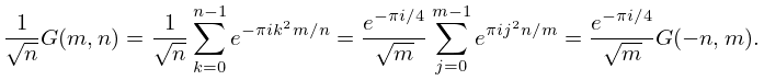
20.11.2

\frac{1}{\sqrt{n}}G(m,n)=\frac{1}{\sqrt{n}}\sum\limits_{k=0}^{n-1}e^{-\pi ik^{% 2}m/n}=\frac{e^{-\pi i/4}}{\sqrt{m}}\sum\limits_{j=0}^{m-1}e^{\pi ij^{2}n/m}=% \frac{e^{-\pi i/4}}{\sqrt{m}}G(-n,m).

ⓘ

Symbols:: $\pi$ : the ratio of the circumference of a circle to its diameter, $\mathrm{e}$ : base of natural logarithm, $\mathrm{i}$ : imaginary unit, $m$ : integer, $n$ : integer and $G(m,n)$ : Gauss sum
Permalink:: http://dlmf.nist.gov/20.11.E2
Encodings:: pMML, png, TeX
See also:: Annotations for §20.11(i), §20.11 and Ch.20

…