hypergeometric differential equation

(0.009 seconds)

11—20 of 81 matching pages

11: 19.18 Derivatives and Differential Equations

… ►

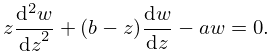
§19.18(ii) Differential Equations

… ►If

n=2

, then elimination of

\partial_{2}v

between (19.18.11) and (19.18.12), followed by the substitution

(b_{1},b_{2},z_{1},z_{2})=(b,c-b,1-z,1)

, produces the Gauss hypergeometric equation (15.10.1). …

12: 13.2 Definitions and Basic Properties

… ►

13.2.1

z\frac{{\mathrm{d}}^{2}w}{{\mathrm{d}z}^{2}}+(b-z)\frac{\mathrm{d}w}{\mathrm{d% }z}-aw=0.

ⓘ

Symbols:: $\frac{\mathrm{d}\NVar{f}}{\mathrm{d}\NVar{x}}$ : derivative of $f$ with respect to $x$ and $z$ : complex variable
A&S Ref:: 13.1.1
Referenced by:: §13.14(i), §13.14(v), §13.2(i), §13.2(v), §13.29(ii), §13.3(i), §13.3(i)
Permalink:: http://dlmf.nist.gov/13.2.E1
Encodings:: pMML, png, TeX
See also:: Annotations for §13.2(i), §13.2(i), §13.2 and Ch.13

… ►It can be regarded as the limiting form of the hypergeometric differential equation (§15.10(i)) that is obtained on replacing

z

\ifrac{z}{b}

, letting

b\to\infty

, and subsequently replacing the symbol

c

b

. In effect, the regular singularities of the hypergeometric differential equation at

b

and

\infty

coalesce into an irregular singularity at

\infty

. …

13: 31.10 Integral Equations and Representations

… ►

31.10.9

\mathcal{K}(\theta,\phi)=P\begin{Bmatrix}0&1&\infty&\\[1.0pt] 0&\frac{1}{2}-\delta-\sigma&\alpha&{\cos}^{2}\theta\\[1.0pt] 1-\gamma&\frac{1}{2}-\epsilon+\sigma&\beta&\end{Bmatrix}\*P\begin{Bmatrix}0&1&% \infty&\\[1.0pt] 0&0&-\frac{1}{2}+\delta+\sigma&{\cos}^{2}\phi\\[1.0pt] 1-\epsilon&1-\delta&-\frac{1}{2}+\epsilon-\sigma&\end{Bmatrix},

… ►

31.10.11

\mathcal{K}(z,t)=(zt-a)^{\frac{1}{2}-\delta-\sigma}\left(\ifrac{zt}{a}\right)^% {-\frac{1}{2}+\delta+\sigma-\alpha}\*{{}_{2}F_{1}}\left({\frac{1}{2}-\delta-% \sigma+\alpha,\frac{3}{2}-\delta-\sigma+\alpha-\gamma\atop\alpha-\beta+1};% \frac{a}{zt}\right)\*P\begin{Bmatrix}0&1&\infty&\\ 0&0&-\frac{1}{2}+\delta+\sigma&\dfrac{(z-a)(t-a)}{(1-a)(zt-a)}\\ 1-\epsilon&1-\delta&-\frac{1}{2}+\epsilon-\sigma&\end{Bmatrix}.

ⓘ

Symbols:: ${{}_{2}F_{1}}\left(\NVar{a},\NVar{b};\NVar{c};\NVar{z}\right)$ : $=F\left(\NVar{a},\NVar{b};\NVar{c};\NVar{z}\right)$ notation for Gauss’ hypergeometric function, $P\NVar{\begin{Bmatrix}\alpha&\beta&\gamma&\\ a_{1}&b_{1}&c_{1}&z\\ a_{2}&b_{2}&c_{2}&\end{Bmatrix}}$ : Riemann’s $P$ -symbol for solutions of the generalized hypergeometric differential equation, $z$ : complex variable, $\gamma$ : real or complex parameter, $\delta$ : real or complex parameter, $\epsilon$ : real or complex parameter, $a$ : complex parameter, $\alpha$ : real or complex parameter, $\beta$ : real or complex parameter, $\mathcal{K}(z,t)$ : kernel and $\sigma$ : separation constant
Permalink:: http://dlmf.nist.gov/31.10.E11
Encodings:: pMML, png, TeX
See also:: Annotations for §31.10(i), §31.10(i), §31.10 and Ch.31

… ►

31.10.22

\mathcal{K}(r,\theta,\phi)=r^{m}{\sin}^{2p}\theta P\begin{Bmatrix}0&1&\infty&% \\ 0&0&a&{\cos}^{2}\theta\\ \tfrac{1}{2}(3-\gamma)&c&b&\end{Bmatrix}\*P\begin{Bmatrix}0&1&\infty&\\ 0&0&a^{\prime}&{\cos}^{2}\phi\\ 1-\epsilon&1-\delta&b^{\prime}&\end{Bmatrix},

…

14: 15.2 Definitions and Analytical Properties

… ►(Both interpretations give solutions of the hypergeometric differential equation (15.10.1), as does

\mathbf{F}\left(a,b;c;z\right)

, which is analytic at

c=0,-1,-2,\dots

.) …

15: 13.29 Methods of Computation

… ►

§13.29(ii) Differential Equations

►A comprehensive and powerful approach is to integrate the differential equations (13.2.1) and (13.14.1) by direct numerical methods. As described in §3.7(ii), to insure stability the integration path must be chosen in such a way that as we proceed along it the wanted solution grows in magnitude at least as fast as all other solutions of the differential equation. ►For

M\left(a,b,z\right)

and

M_{\kappa,\mu}\left(z\right)

this means that in the sector

|\operatorname{ph}z|\leq\pi

we may integrate along outward rays from the origin with initial values obtained from (13.2.2) and (13.14.2). … ►The recurrence relations in §§13.3(i) and 13.15(i) can be used to compute the confluent hypergeometric functions in an efficient way. …

16: 17.6 ${{}_{2}\phi_{1}}$ Function

… ►

§17.6(iv) Differential Equations

…

17: 16.25 Methods of Computation

§16.25 Methods of Computation

►Methods for computing the functions of the present chapter include power series, asymptotic expansions, integral representations, differential equations, and recurrence relations. They are similar to those described for confluent hypergeometric functions, and hypergeometric functions in §§13.29 and 15.19. There is, however, an added feature in the numerical solution of differential equations and difference equations (recurrence relations). …

18: 35.7 Gaussian Hypergeometric Function of Matrix Argument

… ►

§35.7(iii) Partial Differential Equations

… ►Subject to the conditions (a)–(c), the function

f(\mathbf{T})={{}_{2}F_{1}}\left(a,b;c;\mathbf{T}\right)

is the unique solution of each partial differential equation … ►Systems of partial differential equations for the

{{}_{0}F_{1}}

(defined in §35.8) and

{{}_{1}F_{1}}

functions of matrix argument can be obtained by applying (35.8.9) and (35.8.10) to (35.7.9). …

19: Howard S. Cohl

… ►Cohl has published papers in orthogonal polynomials and special functions, and is particularly interested in fundamental solutions of linear partial differential equations on Riemannian manifolds, associated Legendre functions, generalized and basic hypergeometric functions, eigenfunction expansions of fundamental solutions in separable coordinate systems for linear partial differential equations, orthogonal polynomial generating function and generalized expansions, and

q

-series. …

20: Bibliography O

… ►

F. W. J. Olver (1993a) Exponentially-improved asymptotic solutions of ordinary differential equations I: The confluent hypergeometric function. SIAM J. Math. Anal. 24 (3), pp. 756–767.

ⓘ

External Links:: ISSN 0036-1410, Document, MathReview (Hussain S. Nur), ZentralBlatt
Referenced by:: §10.17(v), §13.7(iii), (9.7.18), (9.7.19), (9.7.20), (9.7.21), (9.7.22), (9.7.23), §9.7(v).
Encodings:: BibTeX

…