hyperbolic umbilic catastrophe

SearchAdvancedHelp

(0.004 seconds)

1—10 of 11 matching pages

1: 36.2 Catastrophes and Canonical Integrals

… ►

Normal Forms for Umbilic Catastrophes with Codimension $K=3$

… ►

36.2.3 $${\mathrm{\Phi }}^{(\mathrm{H})}(s,t;𝐱)=s^3+t^3+zst+yt+xs,$$ $𝐱=\{x,y,z\}$,

ⓘ

Defines:

${\mathrm{\Phi }}^{(\mathrm{H})}(s,t;𝐱)$: hyperbolic umbilic catastrophe

Symbols:

$y$: real parameter, $z$: real parameter, $t$: variable, $s$: variable and $x$: real parameter

Referenced by:

§36.10(iii), §36.2(i), §36.8

Permalink:

http://dlmf.nist.gov/36.2.E3

Encodings:

pMML, png, TeX

See also:

Annotations for §36.2(i), §36.2(i), §36.2 and Ch.36

… ►

36.2.5 $\mathrm{U}=\mathrm{E},\mathrm{H}$.

ⓘ

Defines:

${\mathrm{\Psi }}^{(\mathrm{E})}\left(𝐱\right)$: elliptic umbilic canonical integral function, ${\mathrm{\Psi }}^{(\mathrm{H})}\left(𝐱\right)$: hyperbolic umbilic canonical integral function and ${\mathrm{\Psi }}^{(\mathrm{U})}\left(𝐱\right)$: umbilic canonical integral function

Symbols:

$dx$: differential of $x$ , $\exp z$: exponential function, $\mathrm{i}$: imaginary unit, $\int$: integral, : elliptic umbilic catastrophe for $\mathrm{U}=\mathrm{E}\text{ or }\mathrm{K}$ , $t$: variable and $s$: variable

Referenced by:

§36.10(iii), §36.10(iv), §36.2(i), §36.7(iii), §36.8

Permalink:

http://dlmf.nist.gov/36.2.E5

Encodings:

pMML, png, TeX

See also:

Annotations for §36.2(i), §36.2(i), §36.2 and Ch.36

… ►

36.2.11 $\mathrm{U}=\mathrm{E},\mathrm{H}$; $k>0$.

ⓘ

Defines:

${\mathrm{\Psi }}^{(\mathrm{E})}(𝐱;k)$: elliptic umbilic canonical integral function, ${\mathrm{\Psi }}^{(\mathrm{H})}(𝐱;k)$: hyperbolic umbilic canonical integral function and ${\mathrm{\Psi }}^{(\mathrm{U})}(𝐱;k)$: umbilic canonical integral function

Symbols:

$dx$: differential of $x$ , $\exp z$: exponential function, $\mathrm{i}$: imaginary unit, $\int$: integral, : elliptic umbilic catastrophe for $\mathrm{U}=\mathrm{E}\text{ or }\mathrm{K}$ , $k$: variable, $t$: variable and $s$: variable

Referenced by:

§36.2(i)

Permalink:

http://dlmf.nist.gov/36.2.E11

Encodings:

pMML, png, TeX

See also:

Annotations for §36.2(i), §36.2(i), §36.2 and Ch.36

…

2: 36.1 Special Notation

… ►The main functions covered in this chapter are cuspoid catastrophes ${\mathrm{\Phi }}_K(t;𝐱)$; umbilic catastrophes with codimension three ${\mathrm{\Phi }}^{(\mathrm{E})}(s,t;𝐱)$, ${\mathrm{\Phi }}^{(\mathrm{H})}(s,t;𝐱)$; canonical integrals ${\mathrm{\Psi }}_K\left(𝐱\right)$, ${\mathrm{\Psi }}^{(\mathrm{E})}\left(𝐱\right)$, ${\mathrm{\Psi }}^{(\mathrm{H})}\left(𝐱\right)$; diffraction catastrophes ${\mathrm{\Psi }}_K(𝐱;k)$, ${\mathrm{\Psi }}^{(\mathrm{E})}(𝐱;k)$, ${\mathrm{\Psi }}^{(\mathrm{H})}(𝐱;k)$ generated by the catastrophes. …

3: 36.7 Zeros

… ►The zeros of these functions are curves in $𝐱=(x,y,z)$ space; see Nye (2007) for ${\mathrm{\Phi }}_3$ and Nye (2006) for ${\mathrm{\Phi }}^{(\mathrm{H})}$.

4: 36.5 Stokes Sets

… ►

►►

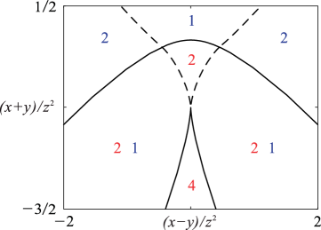
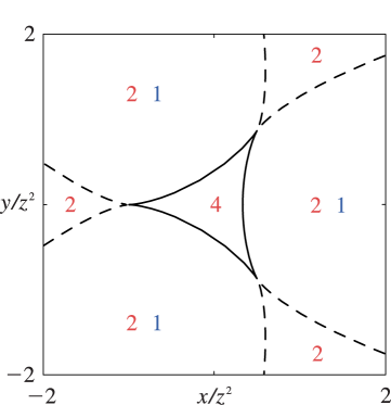
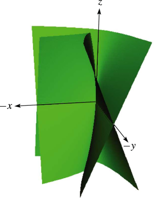
Figure 36.5.5: Elliptic umbilic catastrophe with $z=\mathrm{constant}$. … Magnify

►

►►

Figure 36.5.6: Hyperbolic umbilic catastrophe with $z=\mathrm{constant}$. Magnify

… ►

►►

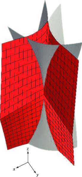
Figure 36.5.9: Sheets of the Stokes surface for the hyperbolic umbilic catastrophe (colored and with mesh) and the bifurcation set (gray). Magnify

5: Bibliography U

… ►

Collisions and umbilic catastrophes. The hyperbolic umbilic canonical diffraction integral. Molecular Phys. 50 (6), pp. 1215–1230.

ⓘ

External Links:

ISSN 0026-8976, Document, MathReview (D. R. J. Chillingworth)

Referenced by:

§36.14(iii).

Encodings:

BibTeX

6: 36.4 Bifurcation Sets

… ►

►►

Figure 36.4.4: Bifurcation set of hyperbolic umbilic catastrophe. Magnify

7: Bibliography N

… ►

Dislocation lines in the hyperbolic umbilic diffraction catastrophe. Proc. Roy. Soc. Lond. Ser. A 462, pp. 2299–2313.

ⓘ

External Links:

ISSN 1364-5021, Document, MathReview, ZentralBlatt

Referenced by:

§36.7(iv).

Encodings:

BibTeX

…

8: 36.6 Scaling Relations

§36.6 Scaling Relations

…

9: 36.10 Differential Equations

… ►In terms of the normal forms (36.2.2) and (36.2.3), the ${\mathrm{\Psi }}^{(\mathrm{U})}\left(𝐱\right)$ satisfy the following operator equations … ►

►

… ►

36.10.15 $$3\frac{{\partial }^2{\mathrm{\Psi }}^{(\mathrm{H})}}{{\partial x}^2}+\mathrm{i}z\frac{\partial {\mathrm{\Psi }}^{(\mathrm{H})}}{\partial y}-x{\mathrm{\Psi }}^{(\mathrm{H})}=0,$$

ⓘ

Symbols:

${\mathrm{\Psi }}^{(\mathrm{H})}\left(𝐱\right)$: hyperbolic umbilic canonical integral function, $\mathrm{i}$: imaginary unit, $\frac{\partial f}{\partial x}$: partial derivative of $f$ with respect to $x$ , $\partial x$: partial differential of $x$ , $y$: real parameter, $z$: real parameter and $x$: real parameter

Permalink:

http://dlmf.nist.gov/36.10.E15

Encodings:

pMML, png, TeX

See also:

Annotations for §36.10(iii), §36.10 and Ch.36

►

36.10.16 $$3\frac{{\partial }^2{\mathrm{\Psi }}^{(\mathrm{H})}}{{\partial y}^2}+\mathrm{i}z\frac{\partial {\mathrm{\Psi }}^{(\mathrm{H})}}{\partial x}-y{\mathrm{\Psi }}^{(\mathrm{H})}=0.$$

ⓘ

Symbols:

${\mathrm{\Psi }}^{(\mathrm{H})}\left(𝐱\right)$: hyperbolic umbilic canonical integral function, $\mathrm{i}$: imaginary unit, $\frac{\partial f}{\partial x}$: partial derivative of $f$ with respect to $x$ , $\partial x$: partial differential of $x$ , $y$: real parameter, $z$: real parameter and $x$: real parameter

Permalink:

http://dlmf.nist.gov/36.10.E16

Encodings:

pMML, png, TeX

See also:

Annotations for §36.10(iii), §36.10 and Ch.36

…

10: 36.11 Leading-Order Asymptotics

§36.11 Leading-Order Asymptotics

… ►

36.11.2 $${\mathrm{\Psi }}_K\left(𝐱\right)=\sqrt{2\pi }\sum _{j=1}^{j_{\max }(𝐱)}\exp \left(\mathrm{i}\left({\mathrm{\Phi }}_K(t_j(𝐱);𝐱)+\frac{1}{4}\pi {(-1)}^{j+K+1}\right)\right){\left|\frac{{\partial }^2{\mathrm{\Phi }}_K(t_j(𝐱);𝐱)}{{\partial t}^2}\right|}^{-1/2}(1+o\left(1\right)).$$

ⓘ

Symbols:

${\mathrm{\Psi }}_K\left(𝐱\right)$: canonical integral function, $\pi$: the ratio of the circumference of a circle to its diameter, ${\mathrm{\Phi }}_K(t;𝐱)$: cuspoid catastrophe of codimension $K$ , $\exp z$: exponential function, $\mathrm{i}$: imaginary unit, $o\left(x\right)$: order less than, $\frac{\partial f}{\partial x}$: partial derivative of $f$ with respect to $x$ , $\partial x$: partial differential of $x$ , $t$: variable, $K$: codimension and $t_j(𝐱)$: solutions

Permalink:

http://dlmf.nist.gov/36.11.E2

Encodings:

pMML, png, TeX

See also:

Annotations for §36.11 and Ch.36

… ►

36.11.7 $${\mathrm{\Psi }}^{(\mathrm{E})}\left(0,0,z\right)=\frac{\pi }{z}\left(\mathrm{i}+\sqrt{3}\exp \left(\frac{4}{27}\mathrm{i}{z}^3\right)+o\left(1\right)\right),$$ $z\to \pm \mathrm{\infty }$,

ⓘ

Symbols:

$\pi$: the ratio of the circumference of a circle to its diameter, ${\mathrm{\Psi }}^{(\mathrm{E})}\left(𝐱\right)$: elliptic umbilic canonical integral function, $\exp z$: exponential function, $\mathrm{i}$: imaginary unit, $o\left(x\right)$: order less than and $z$: real parameter

Permalink:

http://dlmf.nist.gov/36.11.E7

Encodings:

pMML, png, TeX

See also:

Annotations for §36.11, §36.11 and Ch.36

►

36.11.8 $${\mathrm{\Psi }}^{(\mathrm{H})}\left(0,0,z\right)=\frac{2\pi }{z}\left(1-\frac{\mathrm{i}}{\sqrt{3}}\exp \left(\frac{1}{27}\mathrm{i}{z}^3\right)+o\left(1\right)\right),$$ $z\to \pm \mathrm{\infty }$.

ⓘ

Symbols:

$\pi$: the ratio of the circumference of a circle to its diameter, $\exp z$: exponential function, ${\mathrm{\Psi }}^{(\mathrm{H})}\left(𝐱\right)$: hyperbolic umbilic canonical integral function, $\mathrm{i}$: imaginary unit, $o\left(x\right)$: order less than and $z$: real parameter

Permalink:

http://dlmf.nist.gov/36.11.E8

Encodings:

pMML, png, TeX

See also:

Annotations for §36.11, §36.11 and Ch.36