hyperbolic cases

♦ 21—30 of 47 matching pages ♦

(0.002 seconds)

21—30 of 47 matching pages

21: Errata

… ►

Section 4.43

The first paragraph has been rewritten to correct reported errors. The new version is reproduced here.

Let $p$ $(\neq 0)$ and $q$ be real constants and

4.43.1

A=\left(-\tfrac{4}{3}p\right)^{1/2},

B=\left(\tfrac{4}{3}p\right)^{1/2}.

The roots of

4.43.2

z^{3}+pz+q=0

are:

(a)

$A\sin a$ , $A\sin\left(a+\frac{2}{3}\pi\right)$ , and $A\sin\left(a+\frac{4}{3}\pi\right)$ , with $\sin\left(3a\right)=4q/A^{3}$ , when $4p^{3}+27q^{2}\leq 0$ .
(b)

$A\cosh a$ , $A\cosh\left(a+\frac{2}{3}\pi\mathrm{i}\right)$ , and $A\cosh\left(a+\frac{4}{3}\pi\mathrm{i}\right)$ , with $\cosh\left(3a\right)=-4q/A^{3}$ , when $p<0$ , $q<0$ , and $4p^{3}+27q^{2}>0$ .
(c)

$B\sinh a$ , $B\sinh\left(a+\frac{2}{3}\pi\mathrm{i}\right)$ , and $B\sinh\left(a+\frac{4}{3}\pi\mathrm{i}\right)$ , with $\sinh\left(3a\right)=-4q/B^{3}$ , when $p>0$ .

Note that in Case (a) all the roots are real, whereas in Cases (b) and (c) there is one real root and a conjugate pair of complex roots. See also §1.11(iii).

Reported 2014-10-31 by Masataka Urago.

…

22: 19.17 Graphics

… ►The cases

x=0

y=0

correspond to the complete integrals. The case

y=1

corresponds to elementary functions. … ►

See accompanying text — Figure 19.17.8: $R_{J}\left(0,y,1,p\right)$ , $0\leq y\leq 1$ , $-1\leq p\leq 2$ . …See (19.20.10), (19.20.11), and (19.20.8) for the cases $p\to 0\pm$ , $y\to 0+$ , and $y=1$ , respectively. Magnify 3D Help

23: 6.2 Definitions and Interrelations

… ►As in the case of the logarithm (§4.2(i)) there is a cut along the interval

(-\infty,0]

and the principal value is two-valued on

(-\infty,0)

. … ►This is also true of the functions

\operatorname{Ci}\left(z\right)

and

\operatorname{Chi}\left(z\right)

defined in §6.2(ii). … ►

Hyperbolic Analogs of the Sine and Cosine Integrals

►

6.2.15

\operatorname{Shi}\left(z\right)=\int_{0}^{z}\frac{\sinh t}{t}\,\mathrm{d}t,

ⓘ

Defines:: $\operatorname{Shi}\left(\NVar{z}\right)$ : hyperbolic sine integral
Symbols:: $\,\mathrm{d}\NVar{x}$ : differential of $x$ , $\sinh\NVar{z}$ : hyperbolic sine function, $\int$ : integral and $z$ : complex variable
A&S Ref:: 5.2.3
Permalink:: http://dlmf.nist.gov/6.2.E15
Encodings:: pMML, png, TeX
See also:: Annotations for §6.2(ii), §6.2(ii), §6.2 and Ch.6

►

6.2.16

\operatorname{Chi}\left(z\right)=\gamma+\ln z+\int_{0}^{z}\frac{\cosh t-1}{t}% \,\mathrm{d}t.

ⓘ

Defines:: $\operatorname{Chi}\left(\NVar{z}\right)$ : hyperbolic cosine integral
Symbols:: $\gamma$ : Euler’s constant, $\,\mathrm{d}\NVar{x}$ : differential of $x$ , $\cosh\NVar{z}$ : hyperbolic cosine function, $\int$ : integral, $\ln\NVar{z}$ : principal branch of logarithm function and $z$ : complex variable
A&S Ref:: 5.2.4
Referenced by:: §6.4
Permalink:: http://dlmf.nist.gov/6.2.E16
Encodings:: pMML, png, TeX
See also:: Annotations for §6.2(ii), §6.2(ii), §6.2 and Ch.6

…

24: 7.8 Inequalities

… ►

7.8.7

\frac{\sinh x^{2}}{x}<{\mathrm{e}}^{x^{2}}F\left(x\right)=\int_{0}^{x}{\mathrm% {e}}^{t^{2}}\,\mathrm{d}t<\frac{{\mathrm{e}}^{x^{2}}-1}{x},

x>0

ⓘ

Symbols:: $F\left(\NVar{z}\right)$ : Dawson’s integral, $\,\mathrm{d}\NVar{x}$ : differential of $x$ , $\mathrm{e}$ : base of natural logarithm, $\sinh\NVar{z}$ : hyperbolic sine function, $\int$ : integral and $x$ : real variable
Referenced by:: Erratum (V1.1.5) for Additions
Permalink:: http://dlmf.nist.gov/7.8.E7
Encodings:: pMML, png, TeX
Addition (effective with 1.1.5):: A new inequality was added.
See also:: Annotations for §7.8 and Ch.7

… ►

7.8.8

\operatorname{erf}x<\sqrt{1-{\mathrm{e}}^{-4x^{2}/\pi}},

x>0

ⓘ

Symbols:: $\pi$ : the ratio of the circumference of a circle to its diameter, $\operatorname{erf}\NVar{z}$ : error function, $\mathrm{e}$ : base of natural logarithm and $x$ : real variable
Source:: Pólya (1949, (1.5))
Referenced by:: §7.8, Erratum (V1.0.17) for Equation (7.8.8)
Permalink:: http://dlmf.nist.gov/7.8.E8
Encodings:: pMML, png, TeX
Addition (effective with 1.0.17):: This inequality was added. It is Pólya (1949, (1.5)). Note that it is a special case of (8.10.11).
Suggested by Roberto Iacono
See also:: Annotations for §7.8 and Ch.7

25: 19.28 Integrals of Elliptic Integrals

… ►

19.28.8

\int_{0}^{\infty}R_{J}\left(tx,y,z,tp\right)\,\mathrm{d}t=\frac{6}{\sqrt{p}}R_% {C}\left(p,x\right)R_{F}\left(0,y,z\right).

ⓘ

Symbols:: $R_{C}\left(\NVar{x},\NVar{y}\right)$ : Carlson’s combination of inverse circular and inverse hyperbolic functions, $R_{F}\left(\NVar{x},\NVar{y},\NVar{z}\right)$ : symmetric elliptic integral of first kind, $R_{J}\left(\NVar{x},\NVar{y},\NVar{z},\NVar{p}\right)$ : symmetric elliptic integral of third kind, $\,\mathrm{d}\NVar{x}$ : differential of $x$ and $\int$ : integral
Referenced by:: §19.28
Permalink:: http://dlmf.nist.gov/19.28.E8
Encodings:: pMML, png, TeX
See also:: Annotations for §19.28 and Ch.19

… ►

19.28.10

\int_{0}^{\infty}R_{F}\left((ac+bd)^{2},(ad+bc)^{2},4abcd{\cosh}^{2}z\right)\,% \mathrm{d}z=\tfrac{1}{2}R_{F}\left(0,a^{2},b^{2}\right)R_{F}\left(0,c^{2},d^{2% }\right),

a,b,c,d>0

ⓘ

Symbols:: $R_{F}\left(\NVar{x},\NVar{y},\NVar{z}\right)$ : symmetric elliptic integral of first kind, $\,\mathrm{d}\NVar{x}$ : differential of $x$ , $\cosh\NVar{z}$ : hyperbolic cosine function and $\int$ : integral
Referenced by:: §19.28
Permalink:: http://dlmf.nist.gov/19.28.E10
Encodings:: pMML, png, TeX
See also:: Annotations for §19.28 and Ch.19

…

26: 19.11 Addition Theorems

… ►

19.11.5

\Pi\left(\theta,\alpha^{2},k\right)+\Pi\left(\phi,\alpha^{2},k\right)=\Pi\left% (\psi,\alpha^{2},k\right)-\alpha^{2}R_{C}\left(\gamma-\delta,\gamma\right),

ⓘ

Symbols:: $R_{C}\left(\NVar{x},\NVar{y}\right)$ : Carlson’s combination of inverse circular and inverse hyperbolic functions, $\Pi\left(\NVar{\phi},\NVar{\alpha}^{2},\NVar{k}\right)$ : Legendre’s incomplete elliptic integral of the third kind, $\phi$ : real or complex argument, $k$ : real or complex modulus, $\alpha^{2}$ : real or complex parameter, $\theta$ : amplitude, $\psi$ : angle, $\gamma$ and $\delta$
Referenced by:: §19.11(i), §19.11(i), Erratum (V1.0.24) for Subsection 19.11(i)
Permalink:: http://dlmf.nist.gov/19.11.E5
Encodings:: pMML, png, TeX
See also:: Annotations for §19.11(i), §19.11 and Ch.19

… ►In the case of

\theta,\phi\in[0,\pi/2)

and

0\leq k^{2}\leq\alpha^{2}<\min\left(1,\left(1-\cos\theta\cos\phi\cos\psi\right% )^{-1}\right)

, we can use ►

19.11.6_5

R_{C}\left(\gamma-\delta,\gamma\right)=\frac{-1}{\sqrt{\delta}}\operatorname{% arctan}\left(\frac{\sqrt{\delta}\sin\theta\sin\phi\sin\psi}{\alpha^{2}-1-% \alpha^{2}\cos\theta\cos\phi\cos\psi}\right).

ⓘ

Symbols:: $R_{C}\left(\NVar{x},\NVar{y}\right)$ : Carlson’s combination of inverse circular and inverse hyperbolic functions, $\cos\NVar{z}$ : cosine function, $\operatorname{arctan}\NVar{z}$ : arctangent function, $\sin\NVar{z}$ : sine function, $\phi$ : real or complex argument, $\alpha^{2}$ : real or complex parameter, $\theta$ : amplitude, $\psi$ : angle, $\gamma$ and $\delta$
Referenced by:: §19.11(i), Erratum (V1.0.28) for Equations (15.2.3_5), (19.11.6_5)
Permalink:: http://dlmf.nist.gov/19.11.E6_5
Encodings:: pMML, png, TeX
Clarification (effective with 1.0.28):: This equation was given a number.
See also:: Annotations for §19.11(i), §19.11 and Ch.19

… ►

§19.11(ii) Case $\psi=\pi/2$

… ►

19.11.16

\Pi\left(\psi,\alpha^{2},k\right)=2\Pi\left(\theta,\alpha^{2},k\right)+\alpha^% {2}R_{C}\left(\gamma-\delta,\gamma\right),

ⓘ

Symbols:: $R_{C}\left(\NVar{x},\NVar{y}\right)$ : Carlson’s combination of inverse circular and inverse hyperbolic functions, $\Pi\left(\NVar{\phi},\NVar{\alpha}^{2},\NVar{k}\right)$ : Legendre’s incomplete elliptic integral of the third kind, $k$ : real or complex modulus, $\alpha^{2}$ : real or complex parameter, $\theta$ : amplitude, $\delta$ , $\psi$ : angle and $\gamma$
Permalink:: http://dlmf.nist.gov/19.11.E16
Encodings:: pMML, png, TeX
See also:: Annotations for §19.11(iii), §19.11 and Ch.19

…

27: 19.26 Addition Theorems

… ►

19.26.11

R_{C}\left(x+\lambda,y+\lambda\right)+R_{C}\left(x+\mu,y+\mu\right)=R_{C}\left% (x,y\right),

ⓘ

Symbols:: $R_{C}\left(\NVar{x},\NVar{y}\right)$ : Carlson’s combination of inverse circular and inverse hyperbolic functions, $\lambda$ : positive, $x$ : positive, $y$ : positive and $\mu>0$ : parameter
Referenced by:: §19.26(i)
Permalink:: http://dlmf.nist.gov/19.26.E11
Encodings:: pMML, png, TeX
See also:: Annotations for §19.26(i), §19.26 and Ch.19

… ►

19.26.13

R_{C}\left(\alpha^{2},\alpha^{2}-\theta\right)+R_{C}\left(\beta^{2},\beta^{2}-% \theta\right)=R_{C}\left(\sigma^{2},\sigma^{2}-\theta\right),

\sigma=(\alpha\beta+\theta)/(\alpha+\beta)

ⓘ

Symbols:: $R_{C}\left(\NVar{x},\NVar{y}\right)$ : Carlson’s combination of inverse circular and inverse hyperbolic functions and $\alpha^{2}$ : real or complex parameter
Referenced by:: §19.26(i), §19.26(ii)
Permalink:: http://dlmf.nist.gov/19.26.E13
Encodings:: pMML, png, TeX
See also:: Annotations for §19.26(i), §19.26 and Ch.19

… ►

19.26.14

(p-y)R_{C}\left(x,p\right)+(q-y)R_{C}\left(x,q\right)=(\eta-\xi)R_{C}\left(\xi% ,\eta\right),

x\geq 0

y\geq 0

;

p,q\in\mathbb{R}\setminus\{0\}

ⓘ

Symbols:: $R_{C}\left(\NVar{x},\NVar{y}\right)$ : Carlson’s combination of inverse circular and inverse hyperbolic functions, $\in$ : element of, $\mathbb{R}$ : real line, $\setminus$ : set subtraction, $x$ : positive, $y$ : positive, $\xi$ : coordinate and $\eta$ : coordinate
Referenced by:: §19.26(i)
Permalink:: http://dlmf.nist.gov/19.26.E14
Encodings:: pMML, png, TeX
See also:: Annotations for §19.26(i), §19.26 and Ch.19

… ►

§19.26(ii) Case $x=0$

… ►

19.26.25

R_{C}\left(x,y\right)=2R_{C}\left(x+\lambda,y+\lambda\right),

\lambda=y+2\sqrt{x}\sqrt{y}

ⓘ

Symbols:: $R_{C}\left(\NVar{x},\NVar{y}\right)$ : Carlson’s combination of inverse circular and inverse hyperbolic functions, $\lambda$ : positive, $x$ : positive and $y$ : positive
Referenced by:: §19.26(iii)
Permalink:: http://dlmf.nist.gov/19.26.E25
Encodings:: pMML, png, TeX
See also:: Annotations for §19.26(iii), §19.26 and Ch.19

…

28: 28.32 Mathematical Applications

… ►

x=c\cosh\xi\cos\eta,

►

y=c\sinh\xi\sin\eta.

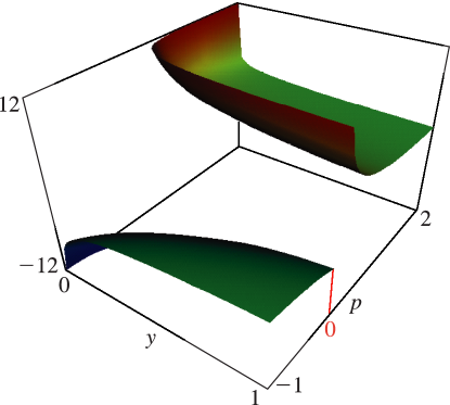
… ►defines a solution of Mathieu’s equation, provided that (in the case of an improper curve) the integral converges with respect to

z

uniformly on compact subsets of

\mathbb{C}

. … ►

x_{1}=\tfrac{1}{2}c\left(\cosh\left(2\alpha\right)+\cos\left(2\beta\right)-% \cosh\left(2\gamma\right)\right),

►

x_{2}=2c\cosh\alpha\cos\beta\sinh\gamma,

…

29: 19.22 Quadratic Transformations

… ►

19.22.20

(p_{\pm}^{2}-p_{\mp}^{2})R_{J}\left(x^{2},y^{2},z^{2},p^{2}\right)=2(p_{\pm}^{% 2}-a^{2})R_{J}\left(a^{2},z_{+}^{2},z_{-}^{2},p_{\pm}^{2}\right)-3R_{F}\left(x% ^{2},y^{2},z^{2}\right)+3R_{C}\left(z^{2},p^{2}\right),

ⓘ

Symbols:: $R_{C}\left(\NVar{x},\NVar{y}\right)$ : Carlson’s combination of inverse circular and inverse hyperbolic functions, $R_{F}\left(\NVar{x},\NVar{y},\NVar{z}\right)$ : symmetric elliptic integral of first kind, $R_{J}\left(\NVar{x},\NVar{y},\NVar{z},\NVar{p}\right)$ : symmetric elliptic integral of third kind and $p_{\pm}$ : modified parameter
Referenced by:: §19.22(i), §19.22(iii), §19.22(iii), §19.36(ii)
Permalink:: http://dlmf.nist.gov/19.22.E20
Encodings:: pMML, png, TeX
See also:: Annotations for §19.22(iii), §19.22 and Ch.19

… ►

19.22.22

R_{C}\left(x^{2},y^{2}\right)=R_{C}\left(a^{2},ay\right).

ⓘ

Symbols:: $R_{C}\left(\NVar{x},\NVar{y}\right)$ : Carlson’s combination of inverse circular and inverse hyperbolic functions
Referenced by:: §19.15, §19.22(iii), §19.22(iii), §19.26(iii)
Permalink:: http://dlmf.nist.gov/19.22.E22
Encodings:: pMML, png, TeX
See also:: Annotations for §19.22(iii), §19.22 and Ch.19

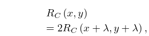
… ►Descending Gauss transformations include, as special cases, transformations of complete integrals into complete integrals; ascending Landen transformations do not. …

30: 10.21 Zeros

… ►The zeros of any cylinder function or its derivative are simple, with the possible exceptions of

z=0

in the case of the functions, and

z=0,\pm\nu

in the case of the derivatives. … ►All of these zeros are simple, provided that

\nu\geq-1

in the case of

J_{\nu}'\left(z\right)

, and

\nu\geq-\tfrac{1}{2}