hyperbolic%20umbilic%20catastrophe
(0.003 seconds)
1—10 of 230 matching pages
1: 4.37 Inverse Hyperbolic Functions
§4.37 Inverse Hyperbolic Functions
… ►The principal values of the inverse hyperbolic cosecant, hyperbolic secant, and hyperbolic tangent are given by … ►Inverse Hyperbolic Sine
… ►Inverse Hyperbolic Cosine
… ►Inverse Hyperbolic Tangent
…2: 36.2 Catastrophes and Canonical Integrals
…
►
Normal Forms Associated with Canonical Integrals: Cuspoid Catastrophe with Codimension
… ►Normal Forms for Umbilic Catastrophes with Codimension
… ►(hyperbolic umbilic). ►Canonical Integrals
… ►Diffraction Catastrophes
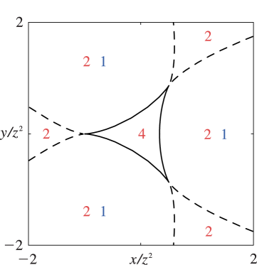
…3: 36.4 Bifurcation Sets
…
►
Critical Points for Umbilics
… ►Bifurcation (Catastrophe) Set for Umbilics
… ►Hyperbolic umbilic bifurcation set (codimension three): … ►Hyperbolic umbilic cusp line (rib): … ►§36.4(ii) Visualizations
…4: 36.5 Stokes Sets
…
►Stokes sets are surfaces (codimension one) in space, across which or acquires an exponentially-small asymptotic contribution (in ), associated with a complex critical point of or .
…
►
► ►
►
Figure 36.5.5: Elliptic umbilic catastrophe with .
…
Magnify
…
§36.5(iii) Umbilics
►Elliptic Umbilic Stokes Set (Codimension three)
… ►Hyperbolic Umbilic Stokes Set (Codimension three)
… ►►
5: 36.1 Special Notation
§36.1 Special Notation
… ►The main functions covered in this chapter are cuspoid catastrophes ; umbilic catastrophes with codimension three , ; canonical integrals , , ; diffraction catastrophes , , generated by the catastrophes. …6: 36.10 Differential Equations
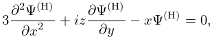
…
►In terms of the normal forms (36.2.2) and (36.2.3), the satisfy the following operator equations
…
►
36.10.14
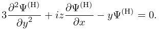
►
36.10.15
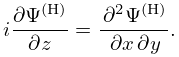
►
36.10.16
…
►
36.10.18
…
7: 36.3 Visualizations of Canonical Integrals
…
►
…
Figure 36.3.9: Modulus of hyperbolic umbilic canonical integral function .
►
…
Figure 36.3.10: Modulus of hyperbolic umbilic canonical integral function .
►
…
Figure 36.3.11: Modulus of hyperbolic umbilic canonical integral function .
►
…
Figure 36.3.12: Modulus of hyperbolic umbilic canonical integral function .
…
►
…
Figure 36.3.18: Phase of hyperbolic umbilic canonical integral .
…
8: 36.6 Scaling Relations
§36.6 Scaling Relations
►Diffraction Catastrophe Scaling
… ►Indices for -Scaling of Magnitude of or (Singularity Index)
… ►9: Bibliography N
…
►
On an integral transform involving a class of Mathieu functions.
SIAM J. Math. Anal. 20 (6), pp. 1500–1513.
…
►
Reduction and evaluation of elliptic integrals.
Math. Comp. 20 (94), pp. 223–231.
…
►
A table of integrals of the error functions.
J. Res. Nat. Bur. Standards Sect B. 73B, pp. 1–20.
…
►
Dislocation lines in the hyperbolic umbilic diffraction catastrophe.
Proc. Roy. Soc. Lond. Ser. A 462, pp. 2299–2313.
►
Dislocation lines in the swallowtail diffraction catastrophe.
Proc. Roy. Soc. Lond. Ser. A 463, pp. 343–355.
