hyperbolic%20functions

SearchAdvancedHelp

(0.004 seconds)

1—10 of 14 matching pages

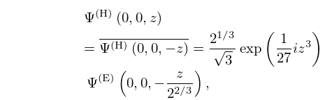
1: 20.10 Integrals

§20.10 Integrals

►

§20.10(i) Mellin Transforms with respect to the Lattice Parameter

… ►Here $\zeta \left(s\right)$ again denotes the Riemann zeta function (§25.2). … ►

§20.10(ii) Laplace Transforms with respect to the Lattice Parameter

… ►For corresponding results for argument derivatives of the theta functions see Erdélyi et al. (1954a, pp. 224–225) or Oberhettinger and Badii (1973, p. 193). …

2: Bibliography B

… ►

Bessel functions and modular relations of higher type and hyperbolic differential equations. Comm. Sém. Math. Univ. Lund [Medd. Lunds Univ. Mat. Sem.] 1952 (Tome Supplementaire), pp. 12–20.

ⓘ

External Links:

MathReview (S. C. van Veen), ZentralBlatt

Referenced by:

§35.5(i).

Encodings:

BibTeX

…

3: 36.2 Catastrophes and Canonical Integrals

… ►

36.2.29 $${\mathrm{\Psi }}^{(\mathrm{H})}\left(0,0,z\right)=\overline{{\mathrm{\Psi }}^{(\mathrm{H})}\left(0,0,-z\right)}=\frac{2^{1/3}}{\sqrt{3}}\exp \left(\frac{1}{27}\mathrm{i}{z}^3\right){\mathrm{\Psi }}^{(\mathrm{E})}\left(0,0,-\frac{z}{2^{2/3}}\right),$$ .

ⓘ

Symbols:

$\overline{z}$: complex conjugate, ${\mathrm{\Psi }}^{(\mathrm{E})}\left(𝐱\right)$: elliptic umbilic canonical integral function, $\exp z$: exponential function, ${\mathrm{\Psi }}^{(\mathrm{H})}\left(𝐱\right)$: hyperbolic umbilic canonical integral function, $\mathrm{i}$: imaginary unit and $z$: real parameter

Referenced by:

Erratum (V1.0.5) for Chapters 8, 20, 36

Permalink:

http://dlmf.nist.gov/36.2.E29

Encodings:

pMML, png, TeX

Addition (effective with 1.0.5):

This equation has been added. For the proof see Berry and Howls (2010).

See also:

Annotations for §36.2(iv), §36.2 and Ch.36

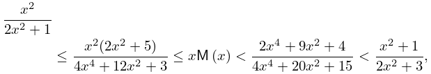
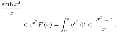
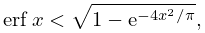
4: 7.8 Inequalities

§7.8 Inequalities

… ►

7.8.5 $x\ge 0$.

ⓘ

Symbols:

$𝖬\left(x\right)$: Mills’ ratio and $x$: real variable

Referenced by:

§7.8

Permalink:

http://dlmf.nist.gov/7.8.E5

Encodings:

pMML, png, TeX

See also:

Annotations for §7.8 and Ch.7

… ►

7.8.7 $x>0$.

ⓘ

Symbols:

$F\left(z\right)$: Dawson’s integral, $dx$: differential of $x$ , $\mathrm{e}$: base of natural logarithm, $\sinh z$: hyperbolic sine function, $\int$: integral and $x$: real variable

Referenced by:

Erratum (V1.1.5) for Additions

Permalink:

http://dlmf.nist.gov/7.8.E7

Encodings:

pMML, png, TeX

Addition (effective with 1.1.5):

A new inequality was added.

See also:

Annotations for §7.8 and Ch.7

►The function $F\left(x\right)/\sqrt{1-{\mathrm{e}}^{-2x^2}}$ is strictly decreasing for $x>0$. … ►

7.8.8 $x>0$.

ⓘ

Symbols:

$\pi$: the ratio of the circumference of a circle to its diameter, $\mathrm{erf}z$: error function, $\mathrm{e}$: base of natural logarithm and $x$: real variable

Source:

Pólya (1949, (1.5))

Referenced by:

§7.8, Erratum (V1.0.17) for Equation (7.8.8)

Permalink:

http://dlmf.nist.gov/7.8.E8

Encodings:

pMML, png, TeX

Addition (effective with 1.0.17):

This inequality was added. It is Pólya (1949, (1.5)). Note that it is a special case of (8.10.11).

Suggested by Roberto Iacono

See also:

Annotations for §7.8 and Ch.7

5: Bibliography F

… ►

ⓘ

Notes:

The “Freely Distributable LIBM” package provides implementations of standard elementary functions plus a few higher functions, e.g. gamma. Double precision, maximum accuracy 20S. Developed by Sun Microsystems.

External Links:

GAMS (package FDLIBM)

Referenced by:

§ ‣ Software Cross Index, § ‣ Software Cross Index.

Encodings:

BibTeX

… ►

Sur certaines sommes des intégral-cosinus. Bull. Soc. Math. Phys. Serbie 12, pp. 13–20 (French).

ⓘ

External Links:

MathReview (L. Carlitz), ZentralBlatt

Referenced by:

§6.15.

Encodings:

BibTeX

… ►

Tables of Elliptic Integrals of the First, Second, and Third Kind. Technical report Technical Report ARL 64-232, Aerospace Research Laboratories, Wright-Patterson Air Force Base, Ohio.

ⓘ

Notes:

Reviewed in Math. Comp. v. 1919(1965)509. Table erratum: Math. Comp. v. 20 (1966), no. 96, pp. 639-640.

Referenced by:

§19.37(ii), §19.37(ii), §19.37(iii), §19.37(iii), §19.37(iii).

Encodings:

BibTeX

… ►

Error bounds for a uniform asymptotic expansion of the Legendre function $Q_n^{-m}(\cosh z)$ . SIAM J. Math. Anal. 21 (2), pp. 523–535.

ⓘ

External Links:

ISSN 0036-1410, Document, MathReview (F. W. J. Olver), ZentralBlatt

Referenced by:

§14.26.

Encodings:

BibTeX

… ►

On weighted polynomial approximation on the whole real axis. Acta Math. Acad. Sci. Hungar. 20, pp. 223–225.

ⓘ

External Links:

ISSN 0001-5954, Document, Link, MathReview (A. K. Varma)

Referenced by:

§18.32.

Encodings:

BibTeX

…

6: 36.4 Bifurcation Sets

… ►

$x=\frac{9}{20}{z}^2.$

… ►

$x=-\frac{3}{20}{z}^2,$

… ►Hyperbolic umbilic bifurcation set (codimension three): … ►Hyperbolic umbilic cusp line (rib): … ►

§36.4(ii) Visualizations

…

7: Bibliography M

… ►

Rational approximations, software and test methods for sine and cosine integrals. Numer. Algorithms 12 (3-4), pp. 259–272.

ⓘ

Notes:

Includes Fortran code, maximum accuracy 20S.

External Links:

ISSN 1017-1398, Document, MathReview, ZentralBlatt

Referenced by:

§6.13, 4th item, §6.21(ii).

Encodings:

BibTeX

… ►

Hill’s Equation. Interscience Tracts in Pure and Applied Mathematics, No. 20, Interscience Publishers John Wiley & Sons, New York-London-Sydney.

ⓘ

Notes:

Reprinted by Dover Publications, Inc., New York, 1979.

External Links:

MathReview (H. Hochstadt), ZentralBlatt

Referenced by:

§1.3(iii), §28.29(i), §28.29(ii), §28.29(ii), §28.29(iii), §28.29(iii), §28.29(iii), §28.30(i), Ch.28, §29.3(i), §29.9.

Encodings:

BibTeX

… ►

Calculation of the modified Bessel functions of the second kind with complex argument. Math. Comp. 20 (95), pp. 407–412.

ⓘ

External Links:

ISSN 0025-5718, FullText, MathReview (H. E. Fettis), ZentralBlatt

Referenced by:

§10.74(iii).

Encodings:

BibTeX

… ►

Hierarchies and logarithmic oscillations in the temporal relaxation patterns of proteins and other complex systems. Proc. Nat. Acad. Sci. U .S. A. 96 (20), pp. 11085–11089.

ⓘ

External Links:

FullText

Referenced by:

§8.24(i).

Encodings:

BibTeX

… ►

The $q$-analogue of the Laguerre polynomials. J. Math. Anal. Appl. 81 (1), pp. 20–47.

ⓘ

External Links:

ISSN 0022-247X, Document, MathReview (R. A. Askey), ZentralBlatt

Referenced by:

§18.27(v).

Encodings:

BibTeX

…

8: Errata

… ►

Scales were corrected in all figures. The interval $-8.4\le \frac{x-y}{\sqrt{2}}\le 8.4$ was replaced by $-12.0\le \frac{x-y}{\sqrt{2}}\le 12.0$ and $-12.7\le \frac{x+y}{\sqrt{2}}\le 4.2$ replaced by $-18.0\le \frac{x+y}{\sqrt{2}}\le 6.0$. All plots and interactive visualizations were regenerated to improve image quality.

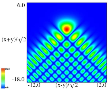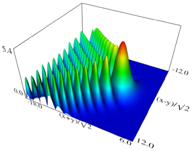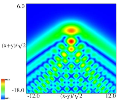
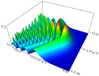
(a) Density plot.	(b) 3D plot.

Figure 36.3.9: Modulus of hyperbolic umbilic canonical integral function $|{\mathrm{\Psi }}^{(\mathrm{H})}\left(x,y,0\right)|$.

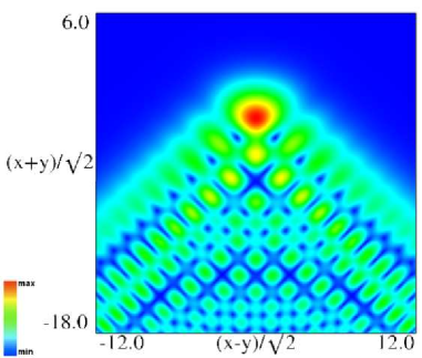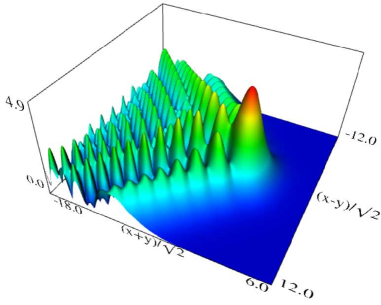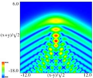
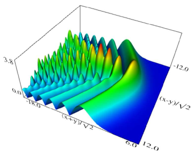
(a) Density plot.	(b) 3D plot.

Figure 36.3.10: Modulus of hyperbolic umbilic canonical integral function $|{\mathrm{\Psi }}^{(\mathrm{H})}\left(x,y,1\right)|$.

(a) Density plot.	(b) 3D plot.

Figure 36.3.11: Modulus of hyperbolic umbilic canonical integral function $|{\mathrm{\Psi }}^{(\mathrm{H})}\left(x,y,2\right)|$.

(a) Density plot.	(b) 3D plot.

Figure 36.3.12: Modulus of hyperbolic umbilic canonical integral function $|{\mathrm{\Psi }}^{(\mathrm{H})}\left(x,y,3\right)|$.

Reported 2016-09-12 by Dan Piponi.

►

The scaling error reported on 2016-09-12 by Dan Piponi also applied to contour and density plots for the phase of the hyperbolic umbilic canonical integrals. Scales were corrected in all figures. The interval $-8.4\le \frac{x-y}{\sqrt{2}}\le 8.4$ was replaced by $-12.0\le \frac{x-y}{\sqrt{2}}\le 12.0$ and $-12.7\le \frac{x+y}{\sqrt{2}}\le 4.2$ replaced by $-18.0\le \frac{x+y}{\sqrt{2}}\le 6.0$. All plots and interactive visualizations were regenerated to improve image quality.

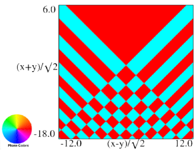(a) Contour plot.	(b) Density plot.

Figure 36.3.18: Phase of hyperbolic umbilic canonical integral $\mathrm{ph}{\mathrm{\Psi }}^{(\mathrm{H})}\left(x,y,0\right)$.

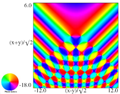(a) Contour plot.	(b) Density plot.

Figure 36.3.19: Phase of hyperbolic umbilic canonical integral $\mathrm{ph}{\mathrm{\Psi }}^{(\mathrm{H})}\left(x,y,1\right)$.

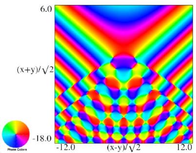(a) Contour plot.	(b) Density plot.

Figure 36.3.20: Phase of hyperbolic umbilic canonical integral $\mathrm{ph}{\mathrm{\Psi }}^{(\mathrm{H})}\left(x,y,2\right)$.

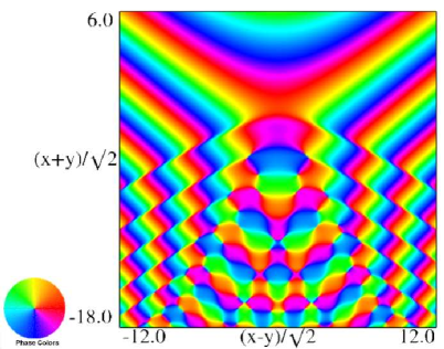(a) Contour plot.	(b) Density plot.

Figure 36.3.21: Phase of hyperbolic umbilic canonical integral $\mathrm{ph}{\mathrm{\Psi }}^{(\mathrm{H})}\left(x,y,3\right)$.

Reported 2016-09-28.

… ►

Several new equations have been added. See (8.17.24), (20.7.34), §20.11(v), (26.12.27), (36.2.28), and (36.2.29).

… ►

Originally the limiting form for $\mathrm{sc}(z,k)$ in the last line of this table was incorrect ($\cosh z$, instead of $\sinh z$).

$\mathrm{sn}(z,k)$ $\to$	$\tanh z$	$\mathrm{cd}(z,k)$ $\to$	$1$	$\mathrm{dc}(z,k)$ $\to$	$1$	$\mathrm{ns}(z,k)$ $\to$	$\coth z$
$\mathrm{cn}(z,k)$ $\to$	$\mathrm{sech}z$	$\mathrm{sd}(z,k)$ $\to$	$\sinh z$	$\mathrm{nc}(z,k)$ $\to$	$\cosh z$	$\mathrm{ds}(z,k)$ $\to$	$\mathrm{csch}z$
$\mathrm{dn}(z,k)$ $\to$	$\mathrm{sech}z$	$\mathrm{nd}(z,k)$ $\to$	$\cosh z$	$\mathrm{sc}(z,k)$ $\to$	$\sinh z$	$\mathrm{cs}(z,k)$ $\to$	$\mathrm{csch}z$

Reported 2010-11-23.

… ►

Bibliographic citations were added in §§1.13(v), 10.14, 10.21(ii), 18.15(v), 18.32, 30.16(iii), 32.13(ii), and as general references in Chapters 19, 20, 22, and 23.

…

9: Software Index

… ► ►►►

	Open Source													With Book						Commercial
…
20 Theta Functions
…

►‘✓’ indicates that a software package implements the functions in a section; ‘a’ indicates available functionality through optional or add-on packages; an empty space indicates no known support. … ►In the list below we identify four main sources of software for computing special functions. … ►

Such software ranges from a collection of reusable software parts (e.g., a library) to fully functional interactive computing environments with an associated computing language. Such software is usually professionally developed, tested, and maintained to high standards. It is available for purchase, often with accompanying updates and consulting support.

… ►The following are web-based software repositories with significant holdings in the area of special functions. …

10: 19.36 Methods of Computation

… ►When the differences are moderately small, the iteration is stopped, the elementary symmetric functions of certain differences are calculated, and a polynomial consisting of a fixed number of terms of the sum in (19.19.7) is evaluated. …where the elementary symmetric functions $E_s$ are defined by (19.19.4). … ►The step from $n$ to $n+1$ is an ascending Landen transformation if $\theta =1$ (leading ultimately to a hyperbolic case of $R_C$) or a descending Gauss transformation if $\theta =-1$ (leading to a circular case of $R_C$). … ►

§19.36(iii) Via Theta Functions

… ►For computation of Legendre’s integral of the third kind, see Abramowitz and Stegun (1964, §§17.7 and 17.8, Examples 15, 17, 19, and 20). …