hyperbolic series for squares

SearchAdvancedHelp

(0.003 seconds)

7 matching pages

1: 22.11 Fourier and Hyperbolic Series

… ►A related hyperbolic series is …

2: 22.16 Related Functions

… ►

22.16.8 $$\mathrm{am}(x,k)=\mathrm{gd}x-\frac{1}{4}k_{}^{\prime }{}_{}{}^2(x-\sinh x\cosh x)\mathrm{sech}x+O\left(k_{}^{\prime }{}_{}{}^4\right).$$

ⓘ

Symbols:

$O\left(x\right)$: order not exceeding, $\mathrm{gd}x$: Gudermannian function, $\mathrm{am}(x,k)$: Jacobi’s amplitude function, $\cosh z$: hyperbolic cosine function, $\mathrm{sech}z$: hyperbolic secant function, $\sinh z$: hyperbolic sine function, $x$: real, $k$: modulus and $k^{\prime }$: complementary modulus

A&S Ref:

16.15.4

Permalink:

http://dlmf.nist.gov/22.16.E8

Encodings:

pMML, png, TeX

See also:

Annotations for §22.16(i), §22.16(i), §22.16 and Ch.22

►

Fourier Series

… ►See Figure 22.16.2. … ►

22.16.26 $$ℰ(x,k)=-{\int }_0^x\left({\mathrm{cs}}^2(t,k)-t^{-2}\right)dt+x^{-1}-\mathrm{cn}(x,k)\mathrm{ds}(x,k).$$

ⓘ

Symbols:

$ℰ(x,k)$: Jacobi’s epsilon function, $\mathrm{cn}(z,k)$: Jacobian elliptic function, $\mathrm{cs}(z,k)$: Jacobian elliptic function, $\mathrm{ds}(z,k)$: Jacobian elliptic function, $dx$: differential of $x$ , $\int$: integral, $x$: real and $k$: modulus

A&S Ref:

16.26.12

Referenced by:

§22.16(ii)

Permalink:

http://dlmf.nist.gov/22.16.E26

Encodings:

pMML, png, TeX

See also:

Annotations for §22.16(ii), §22.16(ii), §22.16 and Ch.22

…

3: 4.38 Inverse Hyperbolic Functions: Further Properties

§4.38 Inverse Hyperbolic Functions: Further Properties

►

§4.38(i) Power Series

… ►

§4.38(ii) Derivatives

►In the following equations square roots have their principal values. … ►All square roots have either possible value.

4: Bibliography S

… ►

On Lindelöf’s error bound for Stirling’s series. J. Reine Angew. Math. 404, pp. 135–139.

ⓘ

External Links:

ISSN 0075-4102, MathReview (Bruce C. Berndt), ZentralBlatt

Referenced by:

§5.11(ii).

Encodings:

BibTeX

… ►

An Introduction to the Operations with Series. 2nd edition, Chelsea Publishing Co., New York.

ⓘ

Notes:

This is a reprint, with corrections, of the first edition [University of Pennsylvania Press, Philadelphia, Pa., 1924].

External Links:

MathReview, ZentralBlatt

Referenced by:

§24.1, §24.6.

Encodings:

BibTeX

… ►

Asymptotic series of generalized Lambert $W$ function. ACM Commun. Comput. Algebra 47 (3), pp. 75–83.

ⓘ

External Links:

FullText, ZentralBlatt

Referenced by:

§4.13, §4.13.

Encodings:

BibTeX

… ►

Algorithm AS 239. Chi-squared and incomplete gamma integral. Appl. Statist. 37 (3), pp. 466–473.

ⓘ

Notes:

Double-precision Fortran.

External Links:

FullText, Code

Referenced by:

5th item.

Encodings:

BibTeX

… ►

An Introduction to Basic Fourier Series. Developments in Mathematics, Vol. 9, Kluwer Academic Publishers, Dordrecht.

ⓘ

External Links:

ISBN 1-4020-1221-7, MathReview (P. D. F. Ion), ZentralBlatt

Referenced by:

§17.3(i).

Encodings:

BibTeX

…

5: 4.45 Methods of Computation

… ►Then we take square roots repeatedly until $|y|$ is sufficiently small, where … ►

Hyperbolic and Inverse Hyperbolic Functions

►The hyperbolic functions can be computed directly from the definitions (4.28.1)–(4.28.7). …For $\mathrm{arccsch}$, $\mathrm{arcsech}$, and $\mathrm{arccoth}$ we have (4.37.7)–(4.37.9). … ►Similarly for the hyperbolic and inverse hyperbolic functions; compare (4.28.1)–(4.28.7), §4.37(iv), and (4.37.7)–(4.37.9). …

6: 19.36 Methods of Computation

… ►The reductions in §19.29(i) represent $x,y,z$ as squares, for example $x=U_{12}^2$ in (19.29.4). … ►The incomplete integrals $R_F(x,y,z)$ and $R_G(x,y,z)$ can be computed by successive transformations in which two of the three variables converge quadratically to a common value and the integrals reduce to $R_C$, accompanied by two quadratically convergent series in the case of $R_G$; compare Carlson (1965, §§5,6). … ►The step from $n$ to $n+1$ is an ascending Landen transformation if $\theta =1$ (leading ultimately to a hyperbolic case of $R_C$) or a descending Gauss transformation if $\theta =-1$ (leading to a circular case of $R_C$). … ►For series expansions of Legendre’s integrals see §19.5. Faster convergence of power series for $K\left(k\right)$ and $E\left(k\right)$ can be achieved by using (19.5.1) and (19.5.2) in the right-hand sides of (19.8.12). …

7: Errata

… ►

Factors inside square roots on the right-hand sides of formulas (19.18.6), (19.20.10), (19.20.19), (19.21.7), (19.21.8), (19.21.10), (19.25.7), (19.25.10) and (19.25.11) were written as products to ensure the correct multivalued behavior.

Reported by Luc Maisonobe on 2021-06-07

… ►

Originally the matrix in the argument of the Gaussian hypergeometric function of matrix argument ${}_2{}^{}F_1^{}$ was written with round brackets. This matrix has been rewritten with square brackets to be consistent with the rest of the DLMF.

… ►

Scales were corrected in all figures. The interval $-8.4\le \frac{x-y}{\sqrt{2}}\le 8.4$ was replaced by $-12.0\le \frac{x-y}{\sqrt{2}}\le 12.0$ and $-12.7\le \frac{x+y}{\sqrt{2}}\le 4.2$ replaced by $-18.0\le \frac{x+y}{\sqrt{2}}\le 6.0$. All plots and interactive visualizations were regenerated to improve image quality.

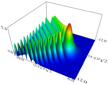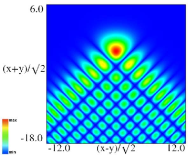
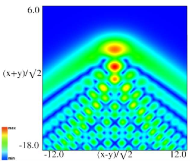
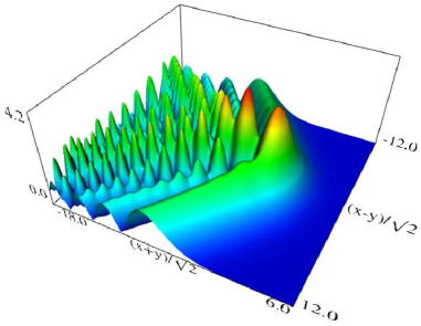
(a) Density plot.	(b) 3D plot.

Figure 36.3.9: Modulus of hyperbolic umbilic canonical integral function $|{\mathrm{\Psi }}^{(\mathrm{H})}\left(x,y,0\right)|$.

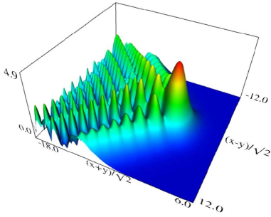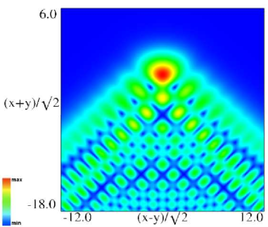
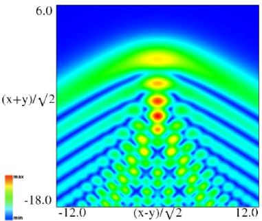
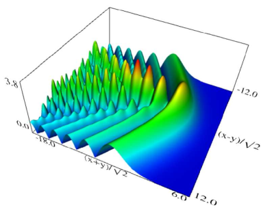
(a) Density plot.	(b) 3D plot.

Figure 36.3.10: Modulus of hyperbolic umbilic canonical integral function $|{\mathrm{\Psi }}^{(\mathrm{H})}\left(x,y,1\right)|$.

(a) Density plot.	(b) 3D plot.

Figure 36.3.11: Modulus of hyperbolic umbilic canonical integral function $|{\mathrm{\Psi }}^{(\mathrm{H})}\left(x,y,2\right)|$.

(a) Density plot.	(b) 3D plot.

Figure 36.3.12: Modulus of hyperbolic umbilic canonical integral function $|{\mathrm{\Psi }}^{(\mathrm{H})}\left(x,y,3\right)|$.

Reported 2016-09-12 by Dan Piponi.

►

The scaling error reported on 2016-09-12 by Dan Piponi also applied to contour and density plots for the phase of the hyperbolic umbilic canonical integrals. Scales were corrected in all figures. The interval $-8.4\le \frac{x-y}{\sqrt{2}}\le 8.4$ was replaced by $-12.0\le \frac{x-y}{\sqrt{2}}\le 12.0$ and $-12.7\le \frac{x+y}{\sqrt{2}}\le 4.2$ replaced by $-18.0\le \frac{x+y}{\sqrt{2}}\le 6.0$. All plots and interactive visualizations were regenerated to improve image quality.

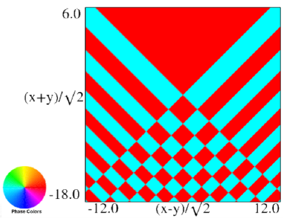(a) Contour plot.	(b) Density plot.

Figure 36.3.18: Phase of hyperbolic umbilic canonical integral $\mathrm{ph}{\mathrm{\Psi }}^{(\mathrm{H})}\left(x,y,0\right)$.

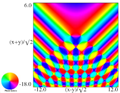(a) Contour plot.	(b) Density plot.

Figure 36.3.19: Phase of hyperbolic umbilic canonical integral $\mathrm{ph}{\mathrm{\Psi }}^{(\mathrm{H})}\left(x,y,1\right)$.

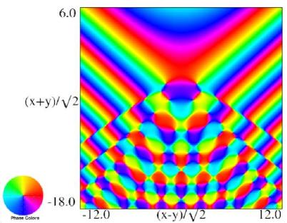(a) Contour plot.	(b) Density plot.

Figure 36.3.20: Phase of hyperbolic umbilic canonical integral $\mathrm{ph}{\mathrm{\Psi }}^{(\mathrm{H})}\left(x,y,2\right)$.

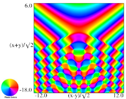(a) Contour plot.	(b) Density plot.

Figure 36.3.21: Phase of hyperbolic umbilic canonical integral $\mathrm{ph}{\mathrm{\Psi }}^{(\mathrm{H})}\left(x,y,3\right)$.

Reported 2016-09-28.

… ►

Originally the limiting form for $\mathrm{sc}(z,k)$ in the last line of this table was incorrect ($\cosh z$, instead of $\sinh z$).

$\mathrm{sn}(z,k)$ $\to$	$\tanh z$	$\mathrm{cd}(z,k)$ $\to$	$1$	$\mathrm{dc}(z,k)$ $\to$	$1$	$\mathrm{ns}(z,k)$ $\to$	$\coth z$
$\mathrm{cn}(z,k)$ $\to$	$\mathrm{sech}z$	$\mathrm{sd}(z,k)$ $\to$	$\sinh z$	$\mathrm{nc}(z,k)$ $\to$	$\cosh z$	$\mathrm{ds}(z,k)$ $\to$	$\mathrm{csch}z$
$\mathrm{dn}(z,k)$ $\to$	$\mathrm{sech}z$	$\mathrm{nd}(z,k)$ $\to$	$\cosh z$	$\mathrm{sc}(z,k)$ $\to$	$\sinh z$	$\mathrm{cs}(z,k)$ $\to$	$\mathrm{csch}z$

Reported 2010-11-23.

…