homogeneous harmonic polynomials

SearchAdvancedHelp

(0.001 seconds)

21—30 of 282 matching pages

21: 18.39 Applications in the Physical Sciences

… ►argument a) The Harmonic Oscillator … ►This is illustrated in Figure 18.39.1 where the first and fourth excited state eigenfunctions of the Schrödinger operator with the rationally extended harmonic potential, of (18.39.19), are shown, and compared with the first and fourth excited states of the harmonic oscillator eigenfunctions of (18.39.14) of paragraph a), above. … ►The eigenfunctions of ${\mathrm{L}}^2$ are the spherical harmonics $Y_{l,m_l}(\theta ,\varphi )$ with eigenvalues ${\mathrm{\hslash }}^{2}l(l+1)$, each with degeneracy $2l+1$ as $m_l=-l,-l+1,\mathrm{\dots },l$. … … ►

The Coulomb–Pollaczek Polynomials

…

22: 2.9 Difference Equations

… ►or equivalently the second-order homogeneous linear difference equation … ►This situation is analogous to second-order homogeneous linear differential equations with an irregular singularity of rank 1 at infinity (§2.7(ii)). … ►For applications of asymptotic methods for difference equations to orthogonal polynomials, see, e. …These methods are particularly useful when the weight function associated with the orthogonal polynomials is not unique or not even known; see, e. …

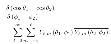
23: 1.17 Integral and Series Representations of the Dirac Delta

… ►

Legendre Polynomials (§§14.7(i) and 18.3)

… ►

Laguerre Polynomials (§18.3)

… ►

Hermite Polynomials (§18.3)

… ►

Spherical Harmonics (§14.30)

►

1.17.25 $$\delta \left(\cos {\theta }_1-\cos {\theta }_2\right)\delta \left({\varphi }_1-{\varphi }_2\right)=\sum _{\mathrm{\ell }=0}^{\mathrm{\infty }}\sum _{m=-\mathrm{\ell }}^{\mathrm{\ell }}{Y}_{\mathrm{\ell },m}({\theta }_1,{\varphi }_1)\overline{Y_{\mathrm{\ell },m}({\theta }_2,{\varphi }_2)}.$$

ⓘ

Symbols:

$\delta \left(x-a\right)$: Dirac delta (or Dirac delta function), $\overline{z}$: complex conjugate, $\cos z$: cosine function, $Y_{l,m}(\theta ,\varphi )$: spherical harmonic and $m$: nonnegative integer

Referenced by:

§1.17(iii)

Permalink:

http://dlmf.nist.gov/1.17.E25

Encodings:

pMML, png, TeX

Notational Change (effective with 1.0.19):

As a notational clarification, the second spherical harmonic in the sum over $\mathrm{\ell }$ has been explicity marked up as a complex conjugate.

See also:

Annotations for §1.17(iii), §1.17(iii), §1.17 and Ch.1

…

24: 3.6 Linear Difference Equations

… ►If $d_n=0$, $\forall n$, then the difference equation is homogeneous; otherwise it is inhomogeneous. … ►

§3.6(ii) Homogeneous Equations

… ►Because the recessive solution of a homogeneous equation is the fastest growing solution in the backward direction, it occurred to J. … ►See also Gautschi (1967) and Gil et al. (2007a, Chapter 4) for the computation of recessive solutions via continued fractions. … ►It is applicable equally to the computation of the recessive solution of the homogeneous equation (3.6.3) or the computation of any solution $w_n$ of the inhomogeneous equation (3.6.1) for which the conditions of §3.6(iv) are satisfied. …

25: Bibliography K

… ►

Nonsymmetric Askey-Wilson polynomials as vector-valued polynomials. Appl. Anal. 90 (3-4), pp. 731–746.

ⓘ

External Links:

ISSN 0003-6811, Link, MathReview (Masatoshi Iida), ZentralBlatt

Referenced by:

§18.38(iii), §18.38(iii).

Encodings:

BibTeX

… ►

The addition formula for Laguerre polynomials. SIAM J. Math. Anal. 8 (3), pp. 535–540.

ⓘ

External Links:

Document, MathReview (M. Mikolas), ZentralBlatt

Referenced by:

(18.14.8), §18.14(i), §18.17(ii), §18.18(ii).

Encodings:

BibTeX

… ►

Meixner-Pollaczek polynomials and the Heisenberg algebra. J. Math. Phys. 30 (4), pp. 767–769.

ⓘ

External Links:

ISSN 0022-2488, Document, MathReview, ZentralBlatt

Referenced by:

§18.21(ii).

Encodings:

BibTeX

… ►

Askey-Wilson polynomial. Scholarpedia 7 (7), pp. 7761.

ⓘ

Notes:

Electronic only

External Links:

Document, FullText

Referenced by:

§18.28(i), §18.28(i).

Encodings:

BibTeX

… ►

An algorithm for solving second order linear homogeneous differential equations. J. Symbolic Comput. 2 (1), pp. 3–43.

ⓘ

External Links:

ISSN 0747-7171, MathReview, ZentralBlatt

Referenced by:

§31.14(ii).

Encodings:

BibTeX

…

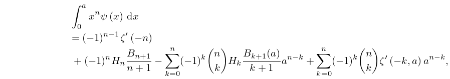
26: 25.11 Hurwitz Zeta Function

… ►For ${\tilde{B}}_n\left(x\right)$ see §24.2(iii). … ►

25.11.14 $$\zeta (-n,a)=-\frac{B_{n+1}\left(a\right)}{n+1},$$ $n=0,1,2,\mathrm{\dots }$.

ⓘ

Symbols:

$B_n\left(x\right)$: Bernoulli polynomials, $\zeta (s,a)$: Hurwitz zeta function, $n$: nonnegative integer and $a$: real or complex parameter

Keywords:

special value

Source:

Apostol (1976, (17), p. 264)

Permalink:

http://dlmf.nist.gov/25.11.E14

Encodings:

pMML, png, TeX

See also:

Annotations for §25.11(v), §25.11 and Ch.25

… ►

25.11.32 $${\int }_0^a{x}^n\psi \left(x\right)dx={(-1)}^{n-1}{\zeta }^{\prime }\left(-n\right)+{(-1)}^n{H}_n\frac{B_{n+1}}{n+1}-\sum _{k=0}^n{(-1)}^k\left(\genfrac{}{}{0.0pt}{}{n}{k}\right)H_k\frac{B_{k+1}(a)}{k+1}{a}^{n-k}+\sum _{k=0}^n{(-1)}^k\left(\genfrac{}{}{0.0pt}{}{n}{k}\right){\zeta }^{\prime }(-k,a)a^{n-k},$$ $n=1,2,\mathrm{\dots }$, $\mathrm{\Re }a>0$,

ⓘ

Symbols:

$B_n$: Bernoulli numbers, $\zeta (s,a)$: Hurwitz zeta function, $\zeta \left(s\right)$: Riemann zeta function, $\left(\genfrac{}{}{0.0pt}{}{m}{n}\right)$: binomial coefficient, $dx$: differential of $x$ , $\psi \left(z\right)$: psi (or digamma) function, $H_n$: harmonic number, $\int$: integral, $\mathrm{\Re }$: real part, $k$: nonnegative integer, $n$: nonnegative integer, $x$: real variable, $a$: real or complex parameter and $h(n)$: harmonic number

Keywords:

definite integral, integral representation

Source:

Adamchik (1998, (17), p. 197)

Referenced by:

Erratum (V1.1.4) for Notation

Permalink:

http://dlmf.nist.gov/25.11.E32

Encodings:

pMML, png, TeX

Notation (effective with 1.1.4):

The notation previously used for the harmonic number $h(n)$ (resp. $h(k)$) has been replaced to be $H_n$ (resp. $H_k$).

Suggested 2021-08-23 by Gergő Nemes

See also:

Annotations for §25.11(viii), §25.11 and Ch.25

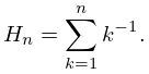
►where $H_n$ are the harmonic numbers: ►

25.11.33 $$H_n=\sum _{k=1}^n{k}^{-1}.$$

ⓘ

Defines:

$H_n$: harmonic number

Symbols:

$k$: nonnegative integer, $n$: nonnegative integer and $h(n)$: harmonic number

Keywords:

harmonic number

Source:

Knuth (1968, Section 1.2.7, p. 73)

Referenced by:

§25.11(viii), §25.16(ii), Erratum (V1.1.4) for Notation

Permalink:

http://dlmf.nist.gov/25.11.E33

Encodings:

pMML, png, TeX

Notation (effective with 1.1.4):

The notation previously used for the harmonic number $h(n)$ has been replaced to be $H_n$.

Suggested 2021-08-23 by Gergő Nemes

See also:

Annotations for §25.11(viii), §25.11 and Ch.25

…

27: Bibliography T

… ►

Zonal Polynomials. Institute of Mathematical Statistics Lecture Notes—Monograph Series, 4, Institute of Mathematical Statistics, Hayward, CA.

ⓘ

External Links:

ISBN 0-940600-05-6, FullText, MathReview (A. W. Davis), ZentralBlatt

Referenced by:

§35.4(i), §35.9.

Encodings:

BibTeX

… ►

Laguerre polynomials: Asymptotics for large degree. Technical report Technical Report AM-R8610, CWI, Amsterdam, The Netherlands.

ⓘ

External Links:

FullText

Referenced by:

§2.4(vi).

Encodings:

BibTeX

… ►

Harmonic Analysis on Symmetric Spaces and Applications. II. Springer-Verlag, Berlin.

ⓘ

External Links:

ISBN 3-540-96663-3, MathReview (Stephen Gelbart), ZentralBlatt

Referenced by:

§35.1, §35.5(ii), Notations K.

Encodings:

BibTeX

… ►

Hyperspherical elliptic harmonics and their relation to the Heun equation. Phys. Rev. A 63 (032510), pp. 1–8.

ⓘ

External Links:

Document

Referenced by:

§31.17(ii).

Encodings:

BibTeX

… ►

Representation Theory and Harmonic Analysis. Contemporary Mathematics, Vol. 191, American Mathematical Society, Providence, RI.

ⓘ

Notes:

Papers from the conference held in honor of Ray A. Kunze at the AMS Special Session, Cincinnati, Ohio, January 12–14, 1994

External Links:

ISBN 0-8218-0310-7, Document, Link, MathReview Entry, ZentralBlatt

Referenced by:

Profile Donald St. P. Richards.

Encodings:

BibTeX

…

28: 21.7 Riemann Surfaces

… ►

21.7.1 $$P(\lambda ,\mu )=0,$$

ⓘ

Symbols:

$P(\lambda ,\mu )$: polynomial

Referenced by:

§21.7(i)

Permalink:

http://dlmf.nist.gov/21.7.E1

Encodings:

pMML, png, TeX

See also:

Annotations for §21.7(i), §21.7 and Ch.21

►where $P(\lambda ,\mu )$ is a polynomial in $\lambda$ and $\mu$ that does not factor over ${ℂ}^2$. …To accomplish this we write (21.7.1) in terms of homogeneous coordinates: … ►

21.7.11 $${\mu }^2=Q(\lambda ),$$

ⓘ

Symbols:

$Q(\lambda )$: polynomial

Permalink:

http://dlmf.nist.gov/21.7.E11

Encodings:

pMML, png, TeX

See also:

Annotations for §21.7(iii), §21.7 and Ch.21

►where $Q(\lambda )$ is a polynomial in $\lambda$ of odd degree $2g+1$ $(\ge 5)$. …

29: 1.2 Elementary Algebra

… ►Let ${\alpha }_1,{\alpha }_2,\mathrm{\dots },{\alpha }_n$ be distinct constants, and $f(x)$ be a polynomial of degree less than $n$. … ►To find the polynomials $f_j(x)$, $j=1,2,\mathrm{\dots },n$, multiply both sides by the denominator of the left-hand side and equate coefficients. … ►

§1.2(iv) Means

… ►The geometric mean $G$ and harmonic mean $H$ of $n$ positive numbers $a_1,a_2,\mathrm{\dots },a_n$ are given by … ►Eigenvalues are the roots of the polynomial equation …

30: 1.10 Functions of a Complex Variable

… ►

Harmonic Functions

►If $u(z)$ is harmonic in $D$, $z_0\in D$, and $u(z)\le u(z_0)$ for all $z\in D$, then $u(z)$ is constant in $D$. Moreover, if $D$ is bounded and $u(z)$ is continuous on $\overline{D}$ and harmonic in $D$, then $u(z)$ is maximum at some point on $\partial D$. … ►Ultraspherical polynomials have generating function …and hence $\frac{d}{dx}{C}_n^{(\lambda )}\left(x\right)=2\lambda C_{n-1}^{(\lambda +1)}\left(x\right)$, that is (18.9.19). …