homogeneous harmonic polynomials

(0.002 seconds)

11—20 of 282 matching pages

11: Tom H. Koornwinder

… ►Koornwinder has published numerous papers on special functions, harmonic analysis, Lie groups, quantum groups, computer algebra, and their interrelations, including an interpretation of Askey–Wilson polynomials on quantum SU(2), and a five-parameter extension (the Macdonald–Koornwinder polynomials) of Macdonald’s polynomials for root systems BC. … ►Koornwinder has been active as an officer in the SIAM Activity Group on Special Functions and Orthogonal Polynomials. … ►

18 Orthogonal Polynomials

…

12: Bibliography M

… ►

T. M. MacRobert (1967) Spherical Harmonics. An Elementary Treatise on Harmonic Functions with Applications. 3rd edition, International Series of Monographs in Pure and Applied Mathematics, Vol. 98, Pergamon Press, Oxford.

ⓘ

External Links:: MathReview (A. Erdélyi), ZentralBlatt
Referenced by:: Ch.14.
Encodings:: BibTeX

… ►

I. Marquette and C. Quesne (2013) New ladder operators for a rational extension of the harmonic oscillator and superintegrability of some two-dimensional systems. J. Math. Phys. 54 (10), pp. Paper 102102, 12 pp..

ⓘ

External Links:: MathReview Entry
Referenced by:: §18.36(vi).
Encodings:: BibTeX

►

I. Marquette and C. Quesne (2016) Connection between quantum systems involving the fourth Painlevé transcendent and

k

-step rational extensions of the harmonic oscillator related to Hermite exceptional orthogonal polynomial. J. Math. Phys. 57 (5), pp. Paper 052101, 15 pp..

ⓘ

External Links:: ISSN 0022-2488, Document, Link, MathReview Entry
Referenced by:: §18.38(iii).
Encodings:: BibTeX

… ►

G. Matviyenko (1993) On the evaluation of Bessel functions. Appl. Comput. Harmon. Anal. 1 (1), pp. 116–135.

ⓘ

External Links:: ISSN 1063-5203, Document, MathReview, ZentralBlatt
Referenced by:: §10.77(iii).
Encodings:: BibTeX

… ►

J. C. P. Miller (1950) On the choice of standard solutions for a homogeneous linear differential equation of the second order. Quart. J. Mech. Appl. Math. 3 (2), pp. 225–235.

ⓘ

External Links:: Document, MathReview (W. R. Wasow), ZentralBlatt
Referenced by:: §12.2(vi), §2.7(iv), §2.7(iv).
Encodings:: BibTeX

…

13: 18.38 Mathematical Applications

… ►

Approximation Theory

… ►

Integrable Systems

… ►

Zonal Spherical Harmonics

►Ultraspherical polynomials are zonal spherical harmonics. … ►

Group Representations

…

14: 29.18 Mathematical Applications

… ►

§29.18(iii) Spherical and Ellipsoidal Harmonics

…

15: 34.3 Basic Properties: $\mathit{3j}$ Symbol

… ►

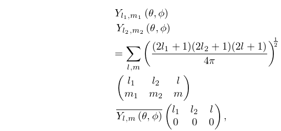
§34.3(vii) Relations to Legendre Polynomials and Spherical Harmonics

►For the polynomials

P_{l}

see §18.3, and for the function

Y_{{l},{m}}

see §14.30. … ►

34.3.20

Y_{{l_{1}},{m_{1}}}\left(\theta,\phi\right)Y_{{l_{2}},{m_{2}}}\left(\theta,% \phi\right)=\sum_{l,m}\left(\frac{(2l_{1}+1)(2l_{2}+1)(2l+1)}{4\pi}\right)^{% \frac{1}{2}}\begin{pmatrix}l_{1}&l_{2}&l\\ m_{1}&m_{2}&m\end{pmatrix}\overline{Y_{{l},{m}}\left(\theta,\phi\right)}\begin% {pmatrix}l_{1}&l_{2}&l\\ 0&0&0\end{pmatrix},

ⓘ

Symbols:: $\pi$ : the ratio of the circumference of a circle to its diameter, $\overline{\NVar{z}}$ : complex conjugate, $Y_{{\NVar{l}},{\NVar{m}}}\left(\NVar{\theta},\NVar{\phi}\right)$ : spherical harmonic, $\begin{pmatrix}\NVar{j_{1}}&\NVar{j_{2}}&\NVar{j_{3}}\\ \NVar{m_{1}}&\NVar{m_{2}}&\NVar{m_{3}}\end{pmatrix}$ : $\mathit{3j}$ symbol and $l,l_{r}$ : non-negative integers or non-negative integers plus one half.
Permalink:: http://dlmf.nist.gov/34.3.E20
Encodings:: pMML, png, TeX
Notational Change (effective with 1.0.19):: As a notational clarification, the spherical harmonic in the sum over $l, m$ has been explicity marked up as a complex conjugate.
See also:: Annotations for §34.3(vii), §34.3 and Ch.34

… ►

34.3.22

\int_{0}^{2\pi}\!\int_{0}^{\pi}Y_{{l_{1}},{m_{1}}}\left(\theta,\phi\right)Y_{{% l_{2}},{m_{2}}}\left(\theta,\phi\right)Y_{{l_{3}},{m_{3}}}\left(\theta,\phi% \right)\sin\theta\,\mathrm{d}\theta\,\mathrm{d}\phi=\left(\frac{(2l_{1}+1)(2l_% {2}+1)(2l_{3}+1)}{4\pi}\right)^{\frac{1}{2}}\begin{pmatrix}l_{1}&l_{2}&l_{3}\\ 0&0&0\end{pmatrix}\begin{pmatrix}l_{1}&l_{2}&l_{3}\\ m_{1}&m_{2}&m_{3}\end{pmatrix}.

ⓘ

Symbols:: $\pi$ : the ratio of the circumference of a circle to its diameter, $\,\mathrm{d}\NVar{x}$ : differential of $x$ , $\int$ : integral, $\sin\NVar{z}$ : sine function, $Y_{{\NVar{l}},{\NVar{m}}}\left(\NVar{\theta},\NVar{\phi}\right)$ : spherical harmonic, $\begin{pmatrix}\NVar{j_{1}}&\NVar{j_{2}}&\NVar{j_{3}}\\ \NVar{m_{1}}&\NVar{m_{2}}&\NVar{m_{3}}\end{pmatrix}$ : $\mathit{3j}$ symbol and $l,l_{r}$ : non-negative integers or non-negative integers plus one half.
Referenced by:: §14.30(ii), §34.3(vii)
Permalink:: http://dlmf.nist.gov/34.3.E22
Encodings:: pMML, png, TeX
See also:: Annotations for §34.3(vii), §34.3 and Ch.34

… ►

16: 3.7 Ordinary Differential Equations

… ►If

h=0

the differential equation is homogeneous, otherwise it is inhomogeneous. … … ►The equations can then be solved by the method of §3.2(ii), if the differential equation is homogeneous, or by Olver’s algorithm (§3.6(v)). … ►This converts the problem into a tridiagonal matrix problem in which the elements of the matrix are polynomials in

\lambda

; compare §3.2(vi). …

17: Bille C. Carlson

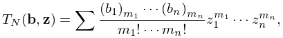
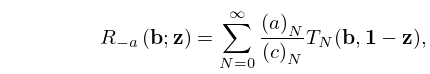
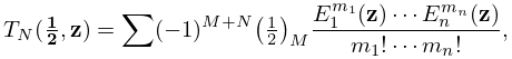
… ►In his paper Lauricella’s hypergeometric function

F_{D}

(1963), he defined the

R

-function, a multivariate hypergeometric function that is homogeneous in its variables, each variable being paired with a parameter. …Also, the homogeneity of the

R

-function has led to a new type of mean value for several variables, accompanied by various inequalities. …

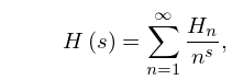
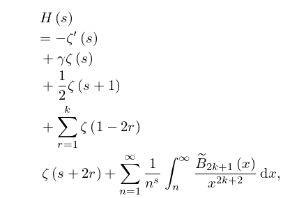
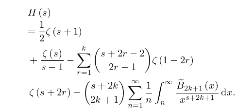
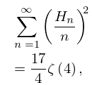
18: 25.16 Mathematical Applications

… ►

25.16.5

H\left(s\right)=\sum_{n=1}^{\infty}\frac{H_{n}}{n^{s}},

ⓘ

Symbols:: $H\left(\NVar{s}\right)$ : Euler sums, $H_{\NVar{n}}$ : harmonic number, $n$ : nonnegative integer, $s$ : complex variable and $h(n)$ : harmonic number
Keywords:: Euler sum, infinite series, series representation
Source:: Apostol and Vu (1984, p. 85)
Referenced by:: Erratum (V1.1.4) for Notation
Permalink:: http://dlmf.nist.gov/25.16.E5
Encodings:: pMML, png, TeX
Notation (effective with 1.1.4):: The notation previously used for the harmonic number $h(n)$ has been replaced to be $H_{n}$ .
Suggested 2021-08-23 by Gergő Nemes
See also:: Annotations for §25.16(ii), §25.16 and Ch.25

►where

H_{n}

is given by (25.11.33). … ►

25.16.6

H\left(s\right)=-\zeta'\left(s\right)+\gamma\zeta\left(s\right)+\frac{1}{2}% \zeta\left(s+1\right)+\sum_{r=1}^{k}\zeta\left(1-2r\right)\zeta\left(s+2r% \right)+\sum_{n=1}^{\infty}\frac{1}{n^{s}}\int_{n}^{\infty}\frac{\widetilde{B}% _{2k+1}\left(x\right)}{x^{2k+2}}\,\mathrm{d}x,

ⓘ

Symbols:: $\gamma$ : Euler’s constant, $H\left(\NVar{s}\right)$ : Euler sums, $\zeta\left(\NVar{s}\right)$ : Riemann zeta function, $\,\mathrm{d}\NVar{x}$ : differential of $x$ , $\int$ : integral, $\widetilde{B}_{\NVar{n}}\left(\NVar{x}\right)$ : periodic Bernoulli functions, $k$ : nonnegative integer, $n$ : nonnegative integer, $x$ : real variable and $s$ : complex variable
Keywords:: Euler sum, finite sum, improper integral, infinite series, integral representation, series representation
Source:: Apostol and Vu (1984, (3), p. 87)
Permalink:: http://dlmf.nist.gov/25.16.E6
Encodings:: pMML, png, TeX
See also:: Annotations for §25.16(ii), §25.16 and Ch.25

►

25.16.7

H\left(s\right)=\frac{1}{2}\zeta\left(s+1\right)+\frac{\zeta\left(s\right)}{s-% 1}-\sum_{r=1}^{k}\genfrac{(}{)}{0.0pt}{}{s+2r-2}{2r-1}\zeta\left(1-2r\right)% \zeta\left(s+2r\right)-\genfrac{(}{)}{0.0pt}{}{s+2k}{2k+1}\sum_{n=1}^{\infty}% \frac{1}{n}\int_{n}^{\infty}\frac{\widetilde{B}_{2k+1}\left(x\right)}{x^{s+2k+% 1}}\,\mathrm{d}x.

ⓘ

Symbols:: $H\left(\NVar{s}\right)$ : Euler sums, $\zeta\left(\NVar{s}\right)$ : Riemann zeta function, $\genfrac{(}{)}{0.0pt}{}{\NVar{m}}{\NVar{n}}$ : binomial coefficient, $\,\mathrm{d}\NVar{x}$ : differential of $x$ , $\int$ : integral, $\widetilde{B}_{\NVar{n}}\left(\NVar{x}\right)$ : periodic Bernoulli functions, $k$ : nonnegative integer, $n$ : nonnegative integer, $x$ : real variable and $s$ : complex variable
Keywords:: Euler sum, finite sum, improper integral, infinite series, integral representation, series representation
Source:: Apostol and Vu (1984, (6), p. 88)
Permalink:: http://dlmf.nist.gov/25.16.E7
Encodings:: pMML, png, TeX
See also:: Annotations for §25.16(ii), §25.16 and Ch.25

… ►

25.16.13

\sum_{n=1}^{\infty}\left(\frac{H_{n}}{n}\right)^{2}=\frac{17}{4}\zeta\left(4% \right),

ⓘ

Symbols:: $\zeta\left(\NVar{s}\right)$ : Riemann zeta function, $H_{\NVar{n}}$ : harmonic number, $n$ : nonnegative integer and $h(n)$ : harmonic number
Keywords:: harmonic number, infinite series, special value
Source:: Flajolet and Salvy (1998, (4-1), p. 24)
Referenced by:: Erratum (V1.1.4) for Notation
Permalink:: http://dlmf.nist.gov/25.16.E13
Encodings:: pMML, png, TeX
Notation (effective with 1.1.4):: The notation previously used for the harmonic number $h(n)$ has been replaced to be $H_{n}$ .
Suggested 2021-08-23 by Gergő Nemes
See also:: Annotations for §25.16(ii), §25.16 and Ch.25

…

19: 3.8 Nonlinear Equations

… ►

§3.8(iv) Zeros of Polynomials

►The polynomial … ►For further information on the computation of zeros of polynomials see McNamee (2007). … ►For describing the distribution of complex zeros of solutions of linear homogeneous second-order differential equations by methods based on the Liouville–Green (WKB) approximation, see Segura (2013). … ►

Example. Wilkinson’s Polynomial

…

20: 19.19 Taylor and Related Series

… ►For

N=0,1,2,\dots

define the homogeneous hypergeometric polynomial ►

19.19.1

T_{N}(\mathbf{b},\mathbf{z})=\sum\frac{{\left(b_{1}\right)_{m_{1}}}\cdots{% \left(b_{n}\right)_{m_{n}}}}{m_{1}!\cdots m_{n}!}z_{1}^{m_{1}}\cdots z_{n}^{m_% {n}},

ⓘ

Symbols:: ${\left(\NVar{a}\right)_{\NVar{n}}}$ : Pochhammer’s symbol (or shifted factorial), $!$ : factorial (as in $n!$ ), $m$ : nonnegative integer, $n$ : nonnegative integer, $N$ : nonnegative integer and $T_{N}(\mathbf{b},\mathbf{z})$ : polynomial
Referenced by:: §19.20(v)
Permalink:: http://dlmf.nist.gov/19.19.E1
Encodings:: pMML, png, TeX
See also:: Annotations for §19.19 and Ch.19

… ►

19.19.2

R_{-a}\left(\mathbf{b};\mathbf{z}\right)=\sum_{N=0}^{\infty}\frac{{\left(a% \right)_{N}}}{{\left(c\right)_{N}}}T_{N}(\mathbf{b},\boldsymbol{{1}}-\mathbf{z% }),

c=\sum_{j=1}^{n}b_{j}

|1-z_{j}|<1

ⓘ

Symbols:: $R_{\NVar{-a}}\left(\NVar{b_{1}},\dots,\NVar{b_{n}};\NVar{z_{1}},\dots,\NVar{z_% {n}}\right)$ or $R_{\NVar{-a}}\left(\NVar{\mathbf{b}};\NVar{\mathbf{z}}\right)$ : multivariate hypergeometric function, ${\left(\NVar{a}\right)_{\NVar{n}}}$ : Pochhammer’s symbol (or shifted factorial), $n$ : nonnegative integer, $N$ : nonnegative integer and $T_{N}(\mathbf{b},\mathbf{z})$ : polynomial
Referenced by:: §19.19
Permalink:: http://dlmf.nist.gov/19.19.E2
Encodings:: pMML, png, TeX
See also:: Annotations for §19.19 and Ch.19

… ►

19.19.5

T_{N}(\mathbf{\tfrac{1}{2}},\mathbf{z})=\sum(-1)^{M+N}{\left(\tfrac{1}{2}% \right)_{M}}\frac{E_{1}^{m_{1}}(\mathbf{z})\cdots E_{n}^{m_{n}}(\mathbf{z})}{m% _{1}!\cdots m_{n}!},

ⓘ

Symbols:: ${\left(\NVar{a}\right)_{\NVar{n}}}$ : Pochhammer’s symbol (or shifted factorial), $!$ : factorial (as in $n!$ ), $m$ : nonnegative integer, $n$ : nonnegative integer, $N$ : nonnegative integer, $T_{N}(\mathbf{b},\mathbf{z})$ : polynomial, $E_{s}(\mathbf{z})$ : symmetric function and $M$ : sum
Referenced by:: §19.19, §19.36(i)
Permalink:: http://dlmf.nist.gov/19.19.E5
Encodings:: pMML, png, TeX
See also:: Annotations for §19.19 and Ch.19

… ►

19.19.7

R_{-a}\left(\boldsymbol{{\tfrac{1}{2}}};\mathbf{z}\right)=A^{-a}\sum_{N=0}^{% \infty}\frac{{\left(a\right)_{N}}}{{\left(\tfrac{1}{2}n\right)_{N}}}T_{N}(% \boldsymbol{{\tfrac{1}{2}}},\mathbf{Z}),

ⓘ

Symbols:: $R_{\NVar{-a}}\left(\NVar{b_{1}},\dots,\NVar{b_{n}};\NVar{z_{1}},\dots,\NVar{z_% {n}}\right)$ or $R_{\NVar{-a}}\left(\NVar{\mathbf{b}};\NVar{\mathbf{z}}\right)$ : multivariate hypergeometric function, ${\left(\NVar{a}\right)_{\NVar{n}}}$ : Pochhammer’s symbol (or shifted factorial), $n$ : nonnegative integer, $N$ : nonnegative integer, $T_{N}(\mathbf{b},\mathbf{z})$ : polynomial, $\mathbf{Z}$ : variable and $A$
Referenced by:: §19.15, §19.36(i), §19.36(i), §19.36(i)
Permalink:: http://dlmf.nist.gov/19.19.E7
Encodings:: pMML, png, TeX
See also:: Annotations for §19.19 and Ch.19

…