higher-order 3nj symbols

(0.002 seconds)

1—10 of 619 matching pages

1: 34.11 Higher-Order $3nj$ Symbols

§34.11 Higher-Order $3nj$ Symbols

►For information on

12j,15j

,…, symbols, see Varshalovich et al. (1988, §10.12) and Yutsis et al. (1962, pp. 62–65 and 122–153).

2: 34.2 Definition: $\mathit{3j}$ Symbol

§34.2 Definition: $\mathit{3j}$ Symbol

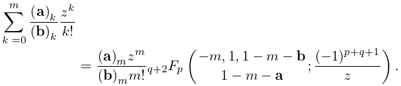
►The quantities

j_{1},j_{2},j_{3}

in the

\mathit{3j}

symbol are called angular momenta. …They therefore satisfy the triangle conditions …The corresponding projective quantum numbers

m_{1},m_{2},m_{3}

are given by … ►When both conditions are satisfied the

\mathit{3j}

symbol can be expressed as the finite sum …

3: Bibliography Q

… ►

F. Qi and J. Mei (1999) Some inequalities of the incomplete gamma and related functions. Z. Anal. Anwendungen 18 (3), pp. 793–799.

ⓘ

External Links:: ISSN 0232-2064, FullText, MathReview (Richard B. Paris), ZentralBlatt
Referenced by:: §8.10.
Encodings:: BibTeX

… ►

S.-L. Qiu and M. K. Vamanamurthy (1996) Sharp estimates for complete elliptic integrals. SIAM J. Math. Anal. 27 (3), pp. 823–834.

ⓘ

External Links:: ISSN 0036-1410, Document, MathReview (G. D. Anderson), ZentralBlatt
Referenced by:: §19.9(i), §19.9(i).
Encodings:: BibTeX

… ►

C. Quesne (2011) Higher-Order SUSY, Exactly Solvable Potentials, and Exceptional Orthogonal Polynomials. Modern Physics Letters A 26, pp. 1843–1852.

ⓘ

External Links:: Document, Link
Referenced by:: §18.38(iii).
Encodings:: BibTeX

4: 24.14 Sums

… ►

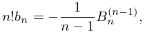
§24.14(i) Quadratic Recurrence Relations

… ►

§24.14(ii) Higher-Order Recurrence Relations

… ►

24.14.10

\sum\frac{(2n)!}{(2j)!(2k)!(2\ell)!(2m)!}B_{2j}B_{2k}B_{2\ell}B_{2m}=-{2n+3% \choose 3}B_{2n}-\frac{4}{3}n^{2}(2n-1)B_{2n-2}.

ⓘ

Symbols:: $B_{\NVar{n}}$ : Bernoulli numbers, $\genfrac{(}{)}{0.0pt}{}{\NVar{m}}{\NVar{n}}$ : binomial coefficient, $!$ : factorial (as in $n!$ ), $j$ : integer, $k$ : integer, $\ell$ : integer, $m$ : integer and $n$ : integer
Referenced by:: §24.14(ii)
Permalink:: http://dlmf.nist.gov/24.14.E10
Encodings:: pMML, png, TeX
See also:: Annotations for §24.14(ii), §24.14 and Ch.24

… ►These identities can be regarded as higher-order recurrences. …

5: 34.4 Definition: $\mathit{6j}$ Symbol

§34.4 Definition: $\mathit{6j}$ Symbol

►The

\mathit{6j}

symbol is defined by the following double sum of products of

\mathit{3j}

symbols: …where the summation is taken over all admissible values of the

m

’s and

m^{\prime}

’s for each of the four

\mathit{3j}

symbols; compare (34.2.2) and (34.2.3). ►Except in degenerate cases the combination of the triangle inequalities for the four

\mathit{3j}

symbols in (34.4.1) is equivalent to the existence of a tetrahedron (possibly degenerate) with edges of lengths

j_{1},j_{2},j_{3},l_{1},l_{2},l_{3}

; see Figure 34.4.1. … ►where

{{}_{4}F_{3}}

is defined as in §16.2. …

6: 34.6 Definition: $\mathit{9j}$ Symbol

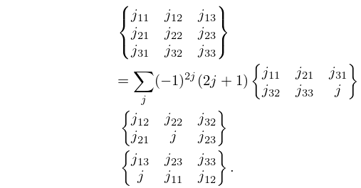
§34.6 Definition: $\mathit{9j}$ Symbol

►The

\mathit{9j}

symbol may be defined either in terms of

\mathit{3j}

symbols or equivalently in terms of

\mathit{6j}

symbols: ►

34.6.1

\begin{Bmatrix}j_{11}&j_{12}&j_{13}\\ j_{21}&j_{22}&j_{23}\\ j_{31}&j_{32}&j_{33}\end{Bmatrix}=\sum_{\mbox{\scriptsize all }m_{rs}}\begin{% pmatrix}j_{11}&j_{12}&j_{13}\\ m_{11}&m_{12}&m_{13}\end{pmatrix}\begin{pmatrix}j_{21}&j_{22}&j_{23}\\ m_{21}&m_{22}&m_{23}\end{pmatrix}\begin{pmatrix}j_{31}&j_{32}&j_{33}\\ m_{31}&m_{32}&m_{33}\end{pmatrix}\*\begin{pmatrix}j_{11}&j_{21}&j_{31}\\ m_{11}&m_{21}&m_{31}\end{pmatrix}\begin{pmatrix}j_{12}&j_{22}&j_{32}\\ m_{12}&m_{22}&m_{32}\end{pmatrix}\begin{pmatrix}j_{13}&j_{23}&j_{33}\\ m_{13}&m_{23}&m_{33}\end{pmatrix},

ⓘ

Defines:: $\begin{Bmatrix}\NVar{j_{11}}&\NVar{j_{12}}&\NVar{j_{13}}\\ \NVar{j_{21}}&\NVar{j_{22}}&\NVar{j_{23}}\\ \NVar{j_{31}}&\NVar{j_{32}}&\NVar{j_{33}}\end{Bmatrix}$ : $\mathit{9j}$ symbol
Symbols:: $\begin{pmatrix}\NVar{j_{1}}&\NVar{j_{2}}&\NVar{j_{3}}\\ \NVar{m_{1}}&\NVar{m_{2}}&\NVar{m_{3}}\end{pmatrix}$ : $\mathit{3j}$ symbol, $j,j_{r}$ : non-negative integers or non-negative integers plus one half., $r$ : nonnegative integer and $s$ : integer
Permalink:: http://dlmf.nist.gov/34.6.E1
Encodings:: pMML, png, TeX
See also:: Annotations for §34.6 and Ch.34

►

34.6.2

\begin{Bmatrix}j_{11}&j_{12}&j_{13}\\ j_{21}&j_{22}&j_{23}\\ j_{31}&j_{32}&j_{33}\end{Bmatrix}=\sum_{j}(-1)^{2j}(2j+1)\begin{Bmatrix}j_{11}% &j_{21}&j_{31}\\ j_{32}&j_{33}&j\end{Bmatrix}\begin{Bmatrix}j_{12}&j_{22}&j_{32}\\ j_{21}&j&j_{23}\end{Bmatrix}\begin{Bmatrix}j_{13}&j_{23}&j_{33}\\ j&j_{11}&j_{12}\end{Bmatrix}.

ⓘ

Symbols:: $\begin{Bmatrix}\NVar{j_{11}}&\NVar{j_{12}}&\NVar{j_{13}}\\ \NVar{j_{21}}&\NVar{j_{22}}&\NVar{j_{23}}\\ \NVar{j_{31}}&\NVar{j_{32}}&\NVar{j_{33}}\end{Bmatrix}$ : $\mathit{9j}$ symbol, $\begin{Bmatrix}\NVar{j_{1}}&\NVar{j_{2}}&\NVar{j_{3}}\\ \NVar{l_{1}}&\NVar{l_{2}}&\NVar{l_{3}}\end{Bmatrix}$ : $\mathit{6j}$ symbol and $j,j_{r}$ : non-negative integers or non-negative integers plus one half.
Referenced by:: §34.13
Permalink:: http://dlmf.nist.gov/34.6.E2
Encodings:: pMML, png, TeX
See also:: Annotations for §34.6 and Ch.34

►The

\mathit{9j}

symbol may also be written as a finite triple sum equivalent to a terminating generalized hypergeometric series of three variables with unit arguments. …

7: Bibliography O

… ►

K. Okamoto (1981) On the

\tau

-function of the Painlevé equations. Phys. D 2 (3), pp. 525–535.

ⓘ

External Links:: ISSN 0167-2789, Document, MathReview (D. A. Lutz), ZentralBlatt
Referenced by:: §32.6(i), §32.6(ii).
Encodings:: BibTeX

… ►

S. Okui (1974) Complete elliptic integrals resulting from infinite integrals of Bessel functions. J. Res. Nat. Bur. Standards Sect. B 78B (3), pp. 113–135.

ⓘ

External Links:: ISSN 0160-1741, MathReview (Y. L. Luke), ZentralBlatt
Referenced by:: §10.22(vi), §10.43(vi).
Encodings:: BibTeX

… ►

A. B. Olde Daalhuis and F. W. J. Olver (1995b) On the calculation of Stokes multipliers for linear differential equations of the second order. Methods Appl. Anal. 2 (3), pp. 348–367.

ⓘ

External Links:: ISSN 1073-2772, Pdf, MathReview (Archibald D. MacGillivray), ZentralBlatt
Referenced by:: §2.7(ii).
Encodings:: BibTeX

… ►

A. B. Olde Daalhuis (1998a) Hyperasymptotic solutions of higher order linear differential equations with a singularity of rank one. Proc. Roy. Soc. London Ser. A 454, pp. 1–29.

ⓘ

External Links:: ISSN 1364-5021, Document, MathReview (Donald A. Lutz), ZentralBlatt
Referenced by:: §2.11(v), §2.7(ii).
Encodings:: BibTeX

… ►

A. B. Olde Daalhuis (2004b) On higher-order Stokes phenomena of an inhomogeneous linear ordinary differential equation. J. Comput. Appl. Math. 169 (1), pp. 235–246.

ⓘ

External Links:: ISSN 0377-0427, Document, MathReview (Jorge Mozo Fernández), ZentralBlatt
Referenced by:: §2.11(iv).
Encodings:: BibTeX

…

8: 24.16 Generalizations

… ►

§24.16(i) Higher-Order Analogs

… ►Also for

\ell=1,2,3,\dotsc

, … ►

24.16.6

n!b_{n}=-\frac{1}{n-1}B^{(n-1)}_{n},

n=2,3,\dots

ⓘ

Symbols:: $!$ : factorial (as in $n!$ ), $B^{(\NVar{\ell})}_{\NVar{n}}\left(\NVar{x}\right)$ : generalized Bernoulli polynomials, $n$ : integer and $b_{n}$
Referenced by:: §24.16(i)
Permalink:: http://dlmf.nist.gov/24.16.E6
Encodings:: pMML, png, TeX
See also:: Annotations for §24.16(i), §24.16(i), §24.16 and Ch.24

… ►Let

\chi_{0}

be the trivial character and

\chi_{4}

the unique (nontrivial) character with

f=4

; that is,

\chi_{4}(1)=1

\chi_{4}(3)=-1

\chi_{4}(2)=\chi_{4}(4)=0

. … ►In no particular order, other generalizations include: Bernoulli numbers and polynomials with arbitrary complex index (Butzer et al. (1992)); Euler numbers and polynomials with arbitrary complex index (Butzer et al. (1994)); q-analogs (Carlitz (1954a), Andrews and Foata (1980)); conjugate Bernoulli and Euler polynomials (Hauss (1997, 1998)); Bernoulli–Hurwitz numbers (Katz (1975)); poly-Bernoulli numbers (Kaneko (1997)); Universal Bernoulli numbers (Clarke (1989));

p

-adic integer order Bernoulli numbers (Adelberg (1996));

p

-adic

q

-Bernoulli numbers (Kim and Kim (1999)); periodic Bernoulli numbers (Berndt (1975b)); cotangent numbers (Girstmair (1990b)); Bernoulli–Carlitz numbers (Goss (1978)); Bernoulli–Padé numbers (Dilcher (2002)); Bernoulli numbers belonging to periodic functions (Urbanowicz (1988)); cyclotomic Bernoulli numbers (Girstmair (1990a)); modified Bernoulli numbers (Zagier (1998)); higher-order Bernoulli and Euler polynomials with multiple parameters (Erdélyi et al. (1953a, §§1.13.1, 1.14.1)).

9: Bibliography H

… ►

P. I. Hadži (1972) Certain sums that contain cylindrical functions. Bul. Akad. Štiince RSS Moldoven. 1972 (3), pp. 75–77, 94 (Russian).

ⓘ

External Links:: MathReview (D. P. Gupta)
Referenced by:: §7.14(iii).
Encodings:: BibTeX

… ►

E. Hille (1929) Note on some hypergeometric series of higher order. J. London Math. Soc. 4, pp. 50–54.

ⓘ

External Links:: Document, ZentralBlatt
Referenced by:: §16.9.
Encodings:: BibTeX

… ►

C. J. Howls, P. J. Langman, and A. B. Olde Daalhuis (2004) On the higher-order Stokes phenomenon. Proc. Roy. Soc. London Ser. A 460, pp. 2285–2303.

ⓘ

External Links:: ISSN 1364-5021, Document, MathReview (W. Balser), ZentralBlatt
Referenced by:: §2.11(iv).
Encodings:: BibTeX

… ►

J. H. Hubbard and B. B. Hubbard (2002) Vector Calculus, Linear Algebra, and Differential Forms: A Unified Approach. 2nd edition, Prentice Hall Inc., Upper Saddle River, NJ.

ⓘ

External Links:: ISBN 0-13-041408-5; 978-0-13-041408-3, MathReview (W. P. Ziemer), ZentralBlatt
Referenced by:: §1.6(i).
Encodings:: BibTeX

… ►

M. N. Huxley (2003) Exponential sums and lattice points. III. Proc. London Math. Soc. (3) 87 (3), pp. 591–609.

ⓘ

External Links:: ISSN 0024-6115, Document, Link, MathReview (Angel V. Kumchev), ZentralBlatt
Referenced by:: §27.11, §27.11, Erratum (V1.1.8) for Section 27.11.
Encodings:: BibTeX

10: 17.8 Special Cases of ${{}_{r}\psi_{r}}$ Functions

… ►

17.8.1

\sum_{n=-\infty}^{\infty}(-z)^{n}q^{n(n-1)/2}=\left(q,z,q/z;q\right)_{\infty};

ⓘ

Symbols:: $\left(\NVar{a_{1},a_{2},\dots,a_{r}};\NVar{q}\right)_{\NVar{n}}$ : multiple $q$ -Pochhammer symbol, $q$ : complex base, $n$ : nonnegative integer and $z$ : complex variable
Referenced by:: §17.8
Permalink:: http://dlmf.nist.gov/17.8.E1
Encodings:: pMML, png, TeX
See also:: Annotations for §17.8, §17.8 and Ch.17

… ►

17.8.3

\sum_{n=-\infty}^{\infty}(-1)^{n}q^{n(3n-1)/2}z^{3n}(1+zq^{n})=\left(q,-z,-q/z% ;q\right)_{\infty}\left(qz^{2},q/{z^{2}};q^{2}\right)_{\infty}.

ⓘ

Symbols:: $\left(\NVar{a_{1},a_{2},\dots,a_{r}};\NVar{q}\right)_{\NVar{n}}$ : multiple $q$ -Pochhammer symbol, $q$ : complex base, $n$ : nonnegative integer and $z$ : complex variable
Referenced by:: §17.8, §17.8, Erratum (V1.2.3) for Additions
Permalink:: http://dlmf.nist.gov/17.8.E3
Encodings:: pMML, png, TeX
See also:: Annotations for §17.8, §17.8 and Ch.17

►Apart from Jacobi’s triple product identity (17.8.1) and the quintuple product identity (17.8.3) (see Cooper (2006) for a review), there also exist higher-order tuple product identities. … ►

17.8.5

{{}_{3}\psi_{3}}\left({b,c,d\atop q/b,q/c,q/d};q,\frac{q}{bcd}\right)=\frac{% \left(q,q/(bc),q/(bd),q/(cd);q\right)_{\infty}}{\left(q/b,q/c,q/d,q/(bcd);q% \right)_{\infty}},

\left|q\right|<\left|bcd\right|

ⓘ

Symbols:: ${{}_{\NVar{r}}\psi_{\NVar{s}}}\left(\NVar{a_{1},\dots,a_{r}};\NVar{b_{1},\dots% ,b_{s}};\NVar{q},\NVar{z}\right)$ or ${{}_{\NVar{r}}\psi_{\NVar{s}}}\left({\NVar{a_{1},\dots,a_{r}}\atop\NVar{b_{1},% \dots,b_{s}}};\NVar{q},\NVar{z}\right)$ : bilateral basic hypergeometric (or bilateral $q$ -hypergeometric) function, $\left(\NVar{a_{1},a_{2},\dots,a_{r}};\NVar{q}\right)_{\NVar{n}}$ : multiple $q$ -Pochhammer symbol and $q$ : complex base
Referenced by:: Erratum (V1.2.1) for Equation (17.8.5)
Permalink:: http://dlmf.nist.gov/17.8.E5
Encodings:: pMML, png, TeX
Correction (effective with 1.2.1):: The constraint $\left|q\right|<\left|bcd\right|$ was added.
See also:: Annotations for §17.8, §17.8 and Ch.17

►

17.8.6

{{}_{4}\psi_{4}}\left({-qa^{\frac{1}{2}},b,c,d\atop-a^{\frac{1}{2}},aq/b,aq/c,% aq/d};q,\frac{qa^{\frac{3}{2}}}{bcd}\right)=\frac{\left(aq,aq/(bc),aq/(bd),aq/% (cd),qa^{\frac{1}{2}}/b,qa^{\frac{1}{2}}/c,qa^{\frac{1}{2}}/d,q,q/a;q\right)_{% \infty}}{\left(aq/b,aq/c,aq/d,q/b,q/c,q/d,qa^{\frac{1}{2}},qa^{-\frac{1}{2}},% qa^{\frac{3}{2}}/(bcd);q\right)_{\infty}},

\left|qa^{\frac{3}{2}}\right|<\left|bcd\right|

ⓘ

Symbols:: ${{}_{\NVar{r}}\psi_{\NVar{s}}}\left(\NVar{a_{1},\dots,a_{r}};\NVar{b_{1},\dots% ,b_{s}};\NVar{q},\NVar{z}\right)$ or ${{}_{\NVar{r}}\psi_{\NVar{s}}}\left({\NVar{a_{1},\dots,a_{r}}\atop\NVar{b_{1},% \dots,b_{s}}};\NVar{q},\NVar{z}\right)$ : bilateral basic hypergeometric (or bilateral $q$ -hypergeometric) function, $\left(\NVar{a_{1},a_{2},\dots,a_{r}};\NVar{q}\right)_{\NVar{n}}$ : multiple $q$ -Pochhammer symbol and $q$ : complex base
Referenced by:: Erratum (V1.2.1) for Equation (17.8.6)
Permalink:: http://dlmf.nist.gov/17.8.E6
Encodings:: pMML, png, TeX
Correction (effective with 1.2.1):: The constraint $\left|qa^{\frac{3}{2}}\right|<\left|bcd\right|$ was added.
See also:: Annotations for §17.8, §17.8 and Ch.17

…

higher-order 3nj symbols

1—10 of 619 matching pages

1: 34.11 Higher-Order 3 ⁢ n ⁢ j Symbols

§34.11 Higher-Order 3 ⁢ n ⁢ j Symbols

2: 34.2 Definition: 3 ⁢ j Symbol

§34.2 Definition: 3 ⁢ j Symbol

3: Bibliography Q

4: 24.14 Sums

§24.14(i) Quadratic Recurrence Relations

§24.14(ii) Higher-Order Recurrence Relations

5: 34.4 Definition: 6 ⁢ j Symbol

§34.4 Definition: 6 ⁢ j Symbol

6: 34.6 Definition: 9 ⁢ j Symbol

§34.6 Definition: 9 ⁢ j Symbol

7: Bibliography O

8: 24.16 Generalizations

§24.16(i) Higher-Order Analogs

9: Bibliography H

10: 17.8 Special Cases of ψ r r Functions

1: 34.11 Higher-Order $3nj$ Symbols

§34.11 Higher-Order $3nj$ Symbols

2: 34.2 Definition: $\mathit{3j}$ Symbol

§34.2 Definition: $\mathit{3j}$ Symbol

5: 34.4 Definition: $\mathit{6j}$ Symbol

§34.4 Definition: $\mathit{6j}$ Symbol

6: 34.6 Definition: $\mathit{9j}$ Symbol

§34.6 Definition: $\mathit{9j}$ Symbol

10: 17.8 Special Cases of ${{}_{r}\psi_{r}}$ Functions