half argument

(0.001 seconds)

11—20 of 22 matching pages

11: 34.2 Definition: $\mathit{3j}$ Symbol

… ►Either all of them are nonnegative integers, or one is a nonnegative integer and the other two are half-odd positive integers. … ►

34.2.1

|j_{r}-j_{s}|\leq j_{t}\leq j_{r}+j_{s},

ⓘ

Symbols:: $j,j_{r}$ : non-negative integers or non-negative integers plus one half., $r\in 1,2,3$ , $t\in 1,2,3$ and $s$ : nonnegative integer
Referenced by:: §34.10, §34.2, §34.3(iv)
Permalink:: http://dlmf.nist.gov/34.2.E1
Encodings:: pMML, png, TeX
See also:: Annotations for §34.2 and Ch.34

… ►

34.2.2

m_{r}=-j_{r},-j_{r}+1,\dots,j_{r}-1,j_{r},

r=1,2,3

ⓘ

Symbols:: $j,j_{r}$ : non-negative integers or non-negative integers plus one half. and $r\in 1,2,3$
Referenced by:: §34.4
Permalink:: http://dlmf.nist.gov/34.2.E2
Encodings:: pMML, png, TeX
See also:: Annotations for §34.2 and Ch.34

… ►and the summation is over all nonnegative integers

s

such that the arguments in the factorials are nonnegative. … ►For alternative expressions for the

\mathit{3j}

symbol, written either as a finite sum or as other terminating generalized hypergeometric series

{{}_{3}F_{2}}

of unit argument, see Varshalovich et al. (1988, §§8.21, 8.24–8.26).

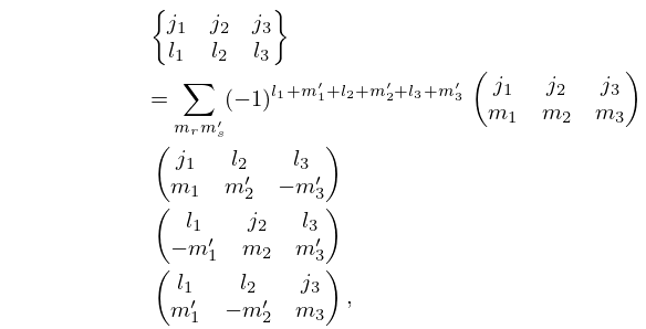
12: 34.6 Definition: $\mathit{9j}$ Symbol

… ►

34.6.1

\begin{Bmatrix}j_{11}&j_{12}&j_{13}\\ j_{21}&j_{22}&j_{23}\\ j_{31}&j_{32}&j_{33}\end{Bmatrix}=\sum_{\mbox{\scriptsize all }m_{rs}}\begin{% pmatrix}j_{11}&j_{12}&j_{13}\\ m_{11}&m_{12}&m_{13}\end{pmatrix}\begin{pmatrix}j_{21}&j_{22}&j_{23}\\ m_{21}&m_{22}&m_{23}\end{pmatrix}\begin{pmatrix}j_{31}&j_{32}&j_{33}\\ m_{31}&m_{32}&m_{33}\end{pmatrix}\*\begin{pmatrix}j_{11}&j_{21}&j_{31}\\ m_{11}&m_{21}&m_{31}\end{pmatrix}\begin{pmatrix}j_{12}&j_{22}&j_{32}\\ m_{12}&m_{22}&m_{32}\end{pmatrix}\begin{pmatrix}j_{13}&j_{23}&j_{33}\\ m_{13}&m_{23}&m_{33}\end{pmatrix},

ⓘ

Defines:: $\begin{Bmatrix}\NVar{j_{11}}&\NVar{j_{12}}&\NVar{j_{13}}\\ \NVar{j_{21}}&\NVar{j_{22}}&\NVar{j_{23}}\\ \NVar{j_{31}}&\NVar{j_{32}}&\NVar{j_{33}}\end{Bmatrix}$ : $\mathit{9j}$ symbol
Symbols:: $\begin{pmatrix}\NVar{j_{1}}&\NVar{j_{2}}&\NVar{j_{3}}\\ \NVar{m_{1}}&\NVar{m_{2}}&\NVar{m_{3}}\end{pmatrix}$ : $\mathit{3j}$ symbol, $j,j_{r}$ : non-negative integers or non-negative integers plus one half., $r$ : nonnegative integer and $s$ : integer
Permalink:: http://dlmf.nist.gov/34.6.E1
Encodings:: pMML, png, TeX
See also:: Annotations for §34.6 and Ch.34

►

34.6.2

\begin{Bmatrix}j_{11}&j_{12}&j_{13}\\ j_{21}&j_{22}&j_{23}\\ j_{31}&j_{32}&j_{33}\end{Bmatrix}=\sum_{j}(-1)^{2j}(2j+1)\begin{Bmatrix}j_{11}% &j_{21}&j_{31}\\ j_{32}&j_{33}&j\end{Bmatrix}\begin{Bmatrix}j_{12}&j_{22}&j_{32}\\ j_{21}&j&j_{23}\end{Bmatrix}\begin{Bmatrix}j_{13}&j_{23}&j_{33}\\ j&j_{11}&j_{12}\end{Bmatrix}.

ⓘ

Symbols:: $\begin{Bmatrix}\NVar{j_{11}}&\NVar{j_{12}}&\NVar{j_{13}}\\ \NVar{j_{21}}&\NVar{j_{22}}&\NVar{j_{23}}\\ \NVar{j_{31}}&\NVar{j_{32}}&\NVar{j_{33}}\end{Bmatrix}$ : $\mathit{9j}$ symbol, $\begin{Bmatrix}\NVar{j_{1}}&\NVar{j_{2}}&\NVar{j_{3}}\\ \NVar{l_{1}}&\NVar{l_{2}}&\NVar{l_{3}}\end{Bmatrix}$ : $\mathit{6j}$ symbol and $j,j_{r}$ : non-negative integers or non-negative integers plus one half.
Referenced by:: §34.13
Permalink:: http://dlmf.nist.gov/34.6.E2
Encodings:: pMML, png, TeX
See also:: Annotations for §34.6 and Ch.34

►The

\mathit{9j}

symbol may also be written as a finite triple sum equivalent to a terminating generalized hypergeometric series of three variables with unit arguments. …

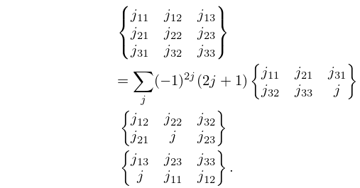
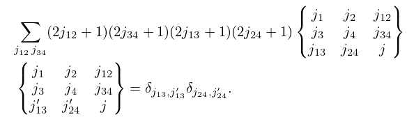
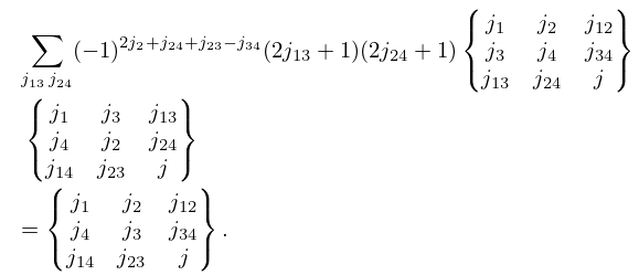
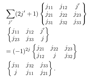
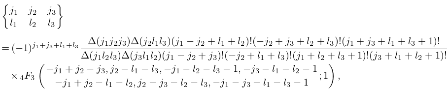
13: 34.7 Basic Properties: $\mathit{9j}$ Symbol

… ►

34.7.1

\begin{Bmatrix}j_{11}&j_{12}&j_{13}\\ j_{21}&j_{22}&j_{13}\\ j_{31}&j_{31}&0\end{Bmatrix}=\frac{(-1)^{j_{12}+j_{21}+j_{13}+j_{31}}}{((2j_{1% 3}+1)(2j_{31}+1))^{\frac{1}{2}}}\begin{Bmatrix}j_{11}&j_{12}&j_{13}\\ j_{22}&j_{21}&j_{31}\end{Bmatrix}.

ⓘ

Symbols:: $\begin{Bmatrix}\NVar{j_{11}}&\NVar{j_{12}}&\NVar{j_{13}}\\ \NVar{j_{21}}&\NVar{j_{22}}&\NVar{j_{23}}\\ \NVar{j_{31}}&\NVar{j_{32}}&\NVar{j_{33}}\end{Bmatrix}$ : $\mathit{9j}$ symbol, $\begin{Bmatrix}\NVar{j_{1}}&\NVar{j_{2}}&\NVar{j_{3}}\\ \NVar{l_{1}}&\NVar{l_{2}}&\NVar{l_{3}}\end{Bmatrix}$ : $\mathit{6j}$ symbol and $j,j_{r}$ : non-negative integers or non-negative integers plus one half.
Permalink:: http://dlmf.nist.gov/34.7.E1
Encodings:: pMML, png, TeX
See also:: Annotations for §34.7(i), §34.7 and Ch.34

… ►Odd permutations of columns or rows introduce a phase factor

(-1)^{R}

, where

R

is the sum of all arguments of the

\mathit{9j}

symbol. … ►

34.7.2

\sum_{j_{12}\,j_{34}}(2j_{12}+1)(2j_{34}+1)(2j_{13}+1)(2j_{24}+1)\begin{% Bmatrix}j_{1}&j_{2}&j_{12}\\ j_{3}&j_{4}&j_{34}\\ j_{13}&j_{24}&j\end{Bmatrix}\begin{Bmatrix}j_{1}&j_{2}&j_{12}\\ j_{3}&j_{4}&j_{34}\\ j^{\prime}_{13}&j^{\prime}_{24}&j\end{Bmatrix}=\delta_{j_{13},j^{\prime}_{13}}% \delta_{j_{24},j^{\prime}_{24}}.

ⓘ

Symbols:: $\delta_{\NVar{j},\NVar{k}}$ : Kronecker delta, $\begin{Bmatrix}\NVar{j_{11}}&\NVar{j_{12}}&\NVar{j_{13}}\\ \NVar{j_{21}}&\NVar{j_{22}}&\NVar{j_{23}}\\ \NVar{j_{31}}&\NVar{j_{32}}&\NVar{j_{33}}\end{Bmatrix}$ : $\mathit{9j}$ symbol and $j,j_{r}$ : non-negative integers or non-negative integers plus one half.
Permalink:: http://dlmf.nist.gov/34.7.E2
Encodings:: pMML, png, TeX
See also:: Annotations for §34.7(iv), §34.7 and Ch.34

… ►

34.7.3

\sum_{j_{13}\,j_{24}}(-1)^{2j_{2}+j_{24}+j_{23}-j_{34}}(2j_{13}+1)(2j_{24}+1)% \begin{Bmatrix}j_{1}&j_{2}&j_{12}\\ j_{3}&j_{4}&j_{34}\\ j_{13}&j_{24}&j\end{Bmatrix}\begin{Bmatrix}j_{1}&j_{3}&j_{13}\\ j_{4}&j_{2}&j_{24}\\ j_{14}&j_{23}&j\end{Bmatrix}=\begin{Bmatrix}j_{1}&j_{2}&j_{12}\\ j_{4}&j_{3}&j_{34}\\ j_{14}&j_{23}&j\end{Bmatrix}.

ⓘ

Symbols:: $\begin{Bmatrix}\NVar{j_{11}}&\NVar{j_{12}}&\NVar{j_{13}}\\ \NVar{j_{21}}&\NVar{j_{22}}&\NVar{j_{23}}\\ \NVar{j_{31}}&\NVar{j_{32}}&\NVar{j_{33}}\end{Bmatrix}$ : $\mathit{9j}$ symbol and $j,j_{r}$ : non-negative integers or non-negative integers plus one half.
Referenced by:: §34.9
Permalink:: http://dlmf.nist.gov/34.7.E3
Encodings:: pMML, png, TeX
See also:: Annotations for §34.7(vi), §34.7 and Ch.34

… ►

34.7.5

\sum_{j^{\prime}}(2j^{\prime}+1)\begin{Bmatrix}j_{11}&j_{12}&j^{\prime}\\ j_{21}&j_{22}&j_{23}\\ j_{31}&j_{32}&j_{33}\end{Bmatrix}\begin{Bmatrix}j_{11}&j_{12}&j^{\prime}\\ j_{23}&j_{33}&j\end{Bmatrix}={(-1)^{2j}}\begin{Bmatrix}j_{21}&j_{22}&j_{23}\\ j_{12}&j&j_{32}\end{Bmatrix}\begin{Bmatrix}j_{31}&j_{32}&j_{33}\\ j&j_{11}&j_{21}\end{Bmatrix}.

ⓘ

Symbols:: $\begin{Bmatrix}\NVar{j_{11}}&\NVar{j_{12}}&\NVar{j_{13}}\\ \NVar{j_{21}}&\NVar{j_{22}}&\NVar{j_{23}}\\ \NVar{j_{31}}&\NVar{j_{32}}&\NVar{j_{33}}\end{Bmatrix}$ : $\mathit{9j}$ symbol, $\begin{Bmatrix}\NVar{j_{1}}&\NVar{j_{2}}&\NVar{j_{3}}\\ \NVar{l_{1}}&\NVar{l_{2}}&\NVar{l_{3}}\end{Bmatrix}$ : $\mathit{6j}$ symbol and $j,j_{r}$ : non-negative integers or non-negative integers plus one half.
Permalink:: http://dlmf.nist.gov/34.7.E5
Encodings:: pMML, png, TeX
See also:: Annotations for §34.7(vi), §34.7 and Ch.34

14: 34.4 Definition: $\mathit{6j}$ Symbol

… ►

34.4.1

\begin{Bmatrix}j_{1}&j_{2}&j_{3}\\ l_{1}&l_{2}&l_{3}\end{Bmatrix}=\sum_{m_{r}m^{\prime}_{s}}(-1)^{l_{1}+m^{\prime% }_{1}+l_{2}+m^{\prime}_{2}+l_{3}+m^{\prime}_{3}}\*\begin{pmatrix}j_{1}&j_{2}&j% _{3}\\ m_{1}&m_{2}&m_{3}\end{pmatrix}\begin{pmatrix}j_{1}&l_{2}&l_{3}\\ m_{1}&m^{\prime}_{2}&-m^{\prime}_{3}\end{pmatrix}\begin{pmatrix}l_{1}&j_{2}&l_% {3}\\ -m^{\prime}_{1}&m_{2}&m^{\prime}_{3}\end{pmatrix}\begin{pmatrix}l_{1}&l_{2}&j_% {3}\\ m^{\prime}_{1}&-m^{\prime}_{2}&m_{3}\end{pmatrix},

ⓘ

Defines:: $\begin{Bmatrix}\NVar{j_{1}}&\NVar{j_{2}}&\NVar{j_{3}}\\ \NVar{l_{1}}&\NVar{l_{2}}&\NVar{l_{3}}\end{Bmatrix}$ : $\mathit{6j}$ symbol
Symbols:: $\begin{pmatrix}\NVar{j_{1}}&\NVar{j_{2}}&\NVar{j_{3}}\\ \NVar{m_{1}}&\NVar{m_{2}}&\NVar{m_{3}}\end{pmatrix}$ : $\mathit{3j}$ symbol, $j,j_{r}$ : non-negative integers or non-negative integers plus one half., $l,l_{r}$ : non-negative integers or non-negative integers plus one half. and $r$ : nonnegative integer
Referenced by:: §34.10, §34.4, §34.9
Permalink:: http://dlmf.nist.gov/34.4.E1
Encodings:: pMML, png, TeX
See also:: Annotations for §34.4 and Ch.34

… ►

34.4.2

\begin{Bmatrix}j_{1}&j_{2}&j_{3}\\ l_{1}&l_{2}&l_{3}\end{Bmatrix}=\Delta(j_{1}j_{2}j_{3})\Delta(j_{1}l_{2}l_{3})% \Delta(l_{1}j_{2}l_{3})\Delta(l_{1}l_{2}j_{3})\*\sum_{s}\frac{(-1)^{s}(s+1)!}{% (s-j_{1}-j_{2}-j_{3})!(s-j_{1}-l_{2}-l_{3})!(s-l_{1}-j_{2}-l_{3})!(s-l_{1}-l_{% 2}-j_{3})!}\*\frac{1}{(j_{1}+j_{2}+l_{1}+l_{2}-s)!(j_{2}+j_{3}+l_{2}+l_{3}-s)!% (j_{3}+j_{1}+l_{3}+l_{1}-s)!},

ⓘ

Symbols:: $!$ : factorial (as in $n!$ ), $\begin{Bmatrix}\NVar{j_{1}}&\NVar{j_{2}}&\NVar{j_{3}}\\ \NVar{l_{1}}&\NVar{l_{2}}&\NVar{l_{3}}\end{Bmatrix}$ : $\mathit{6j}$ symbol, $j,j_{r}$ : non-negative integers or non-negative integers plus one half., $l,l_{r}$ : non-negative integers or non-negative integers plus one half. and $\Delta(j_{1}j_{2}j_{3})$ : product
Referenced by:: Erratum (V1.0.7) for Equation (34.4.2)
Permalink:: http://dlmf.nist.gov/34.4.E2
Encodings:: pMML, png, TeX
Errata (effective with 1.0.7):: Originally the factor $\Delta(j_{1}j_{2}j_{3})\Delta(j_{1}l_{2}l_{3})\Delta(l_{1}j_{2}l_{3})\Delta(l_% {1}l_{2}j_{3})$ was missing in this equation.
Reported 2012-12-31 by Yu Lin
See also:: Annotations for §34.4 and Ch.34

►where the summation is over all nonnegative integers

s

such that the arguments in the factorials are nonnegative. … ►

34.4.3

\begin{Bmatrix}j_{1}&j_{2}&j_{3}\\ l_{1}&l_{2}&l_{3}\end{Bmatrix}={(-1)^{j_{1}+j_{3}+l_{1}+l_{3}}}\frac{\Delta(j_% {1}j_{2}j_{3})\Delta(j_{2}l_{1}l_{3})(j_{1}-j_{2}+l_{1}+l_{2})!(-j_{2}+j_{3}+l% _{2}+l_{3})!(j_{1}+j_{3}+l_{1}+l_{3}+1)!}{\Delta(j_{1}l_{2}l_{3})\Delta(j_{3}l% _{1}l_{2})(j_{1}-j_{2}+j_{3})!(-j_{2}+l_{1}+l_{3})!(j_{1}+l_{2}+l_{3}+1)!(j_{3% }+l_{1}+l_{2}+1)!}\*{{}_{4}F_{3}}\left({-j_{1}+j_{2}-j_{3},j_{2}-l_{1}-l_{3},-% j_{1}-l_{2}-l_{3}-1,-j_{3}-l_{1}-l_{2}-1\atop-j_{1}+j_{2}-l_{1}-l_{2},j_{2}-j_% {3}-l_{2}-l_{3},-j_{1}-j_{3}-l_{1}-l_{3}-1};1\right),

ⓘ

Symbols:: ${{}_{\NVar{p}}F_{\NVar{q}}}\left(\NVar{a_{1},\dots,a_{p}};\NVar{b_{1},\dots,b_% {q}};\NVar{z}\right)$ or ${{}_{\NVar{p}}F_{\NVar{q}}}\left({\NVar{a_{1},\dots,a_{p}}\atop\NVar{b_{1},% \dots,b_{q}}};\NVar{z}\right)$ : alternatively ${{}_{\NVar{p}}F_{\NVar{q}}}\left(\NVar{\mathbf{a}};\NVar{\mathbf{b}};\NVar{z}\right)$ or ${{}_{\NVar{p}}F_{\NVar{q}}}\left({\NVar{\mathbf{a}}\atop\NVar{\mathbf{b}}};% \NVar{z}\right)$
generalized hypergeometric function, $!$ : factorial (as in $n!$ ), $\begin{Bmatrix}\NVar{j_{1}}&\NVar{j_{2}}&\NVar{j_{3}}\\ \NVar{l_{1}}&\NVar{l_{2}}&\NVar{l_{3}}\end{Bmatrix}$ : $\mathit{6j}$ symbol, $j,j_{r}$ : non-negative integers or non-negative integers plus one half., $l,l_{r}$ : non-negative integers or non-negative integers plus one half. and $\Delta(j_{1}j_{2}j_{3})$ : product
Referenced by:: §18.38(iii)
Permalink:: http://dlmf.nist.gov/34.4.E3
Encodings:: pMML, png, TeX
See also:: Annotations for §34.4 and Ch.34

… ►For alternative expressions for the

\mathit{6j}

symbol, written either as a finite sum or as other terminating generalized hypergeometric series

{{}_{4}F_{3}}

of unit argument, see Varshalovich et al. (1988, §§9.2.1, 9.2.3).

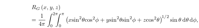
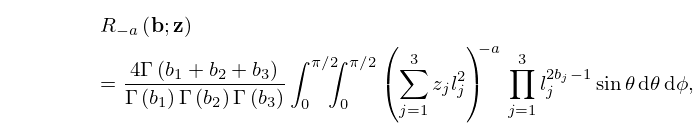
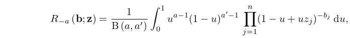
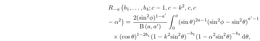
15: 19.23 Integral Representations

… ►

19.23.6

4\pi R_{F}\left(x,y,z\right)=\int_{0}^{2\pi}\!\!\!\!\int_{0}^{\pi}\frac{\sin% \theta\,\mathrm{d}\theta\,\mathrm{d}\phi}{(x{\sin}^{2}\theta{\cos}^{2}\phi+y{% \sin}^{2}\theta{\sin}^{2}\phi+z{\cos}^{2}\theta)^{1/2}},

ⓘ

Symbols:: $R_{F}\left(\NVar{x},\NVar{y},\NVar{z}\right)$ : symmetric elliptic integral of first kind, $\pi$ : the ratio of the circumference of a circle to its diameter, $\cos\NVar{z}$ : cosine function, $\,\mathrm{d}\NVar{x}$ : differential of $x$ , $\int$ : integral, $\sin\NVar{z}$ : sine function and $\phi$ : real or complex argument
Referenced by:: §19.16(ii), §19.23
Permalink:: http://dlmf.nist.gov/19.23.E6
Encodings:: pMML, png, TeX
See also:: Annotations for §19.23 and Ch.19

►

19.23.6_5

R_{G}\left(x,y,z\right)=\frac{1}{4\pi}\int_{0}^{2\pi}\!\!\!\!\int_{0}^{\pi}% \left(x{\sin}^{2}\theta{\cos}^{2}\phi+y{\sin}^{2}\theta{\sin}^{2}\phi+z{\cos}^% {2}\theta\right)^{1/2}\sin\theta\,\mathrm{d}\theta\,\mathrm{d}\phi,

ⓘ

Symbols:: $R_{G}\left(\NVar{x},\NVar{y},\NVar{z}\right)$ : symmetric elliptic integral of second kind, $\pi$ : the ratio of the circumference of a circle to its diameter, $\cos\NVar{z}$ : cosine function, $\,\mathrm{d}\NVar{x}$ : differential of $x$ , $\int$ : integral, $\sin\NVar{z}$ : sine function and $\phi$ : real or complex argument
Referenced by:: (19.16.3), (19.16.3), §19.16(i), §19.16(ii), §19.16(ii), §19.20(ii), §19.23, §19.23, §19.25(vi), Erratum (V1.1.0) for Rearrangement
Permalink:: http://dlmf.nist.gov/19.23.E6_5
Encodings:: pMML, png, TeX
Rearrangement (effective with 1.1.0):: This equation, which was originally (19.16.3), was moved here.
See also:: Annotations for §19.23 and Ch.19

… ►

19.23.9

R_{-a}\left(\mathbf{b};\mathbf{z}\right)=\frac{4\Gamma\left(b_{1}+b_{2}+b_{3}% \right)}{\Gamma\left(b_{1}\right)\Gamma\left(b_{2}\right)\Gamma\left(b_{3}% \right)}\int_{0}^{\pi/2}\!\!\!\!\int_{0}^{\pi/2}\left(\sum_{j=1}^{3}z_{j}l_{j}% ^{2}\right)^{-a}\*\prod_{j=1}^{3}l_{j}^{2b_{j}-1}\sin\theta\,\mathrm{d}\theta% \,\mathrm{d}\phi,

b_{j}>0

\Re z_{j}>0

ⓘ

Symbols:: $R_{\NVar{-a}}\left(\NVar{b_{1}},\dots,\NVar{b_{n}};\NVar{z_{1}},\dots,\NVar{z_% {n}}\right)$ or $R_{\NVar{-a}}\left(\NVar{\mathbf{b}};\NVar{\mathbf{z}}\right)$ : multivariate hypergeometric function, $\Gamma\left(\NVar{z}\right)$ : gamma function, $\pi$ : the ratio of the circumference of a circle to its diameter, $\,\mathrm{d}\NVar{x}$ : differential of $x$ , $\int$ : integral, $\Re$ : real part, $\sin\NVar{z}$ : sine function, $l$ : nonnegative integer and $\phi$ : real or complex argument
Referenced by:: §19.23, §19.23
Permalink:: http://dlmf.nist.gov/19.23.E9
Encodings:: pMML, png, TeX
See also:: Annotations for §19.23 and Ch.19

►

19.23.10

R_{-a}\left(\mathbf{b};\mathbf{z}\right)=\frac{1}{\mathrm{B}\left(a,a^{\prime}% \right)}\int_{0}^{1}u^{a-1}(1-u)^{a^{\prime}-1}\*\prod_{j=1}^{n}(1-u+uz_{j})^{% -b_{j}}\,\mathrm{d}u,

a,a^{\prime}>0

;

a+a^{\prime}=\sum_{j=1}^{n}b_{j}

;

z_{j}\in\mathbb{C}\setminus(-\infty,0]

ⓘ

Symbols:: $R_{\NVar{-a}}\left(\NVar{b_{1}},\dots,\NVar{b_{n}};\NVar{z_{1}},\dots,\NVar{z_% {n}}\right)$ or $R_{\NVar{-a}}\left(\NVar{\mathbf{b}};\NVar{\mathbf{z}}\right)$ : multivariate hypergeometric function, $\mathrm{B}\left(\NVar{a},\NVar{b}\right)$ : beta function, $\mathbb{C}$ : complex plane, $\,\mathrm{d}\NVar{x}$ : differential of $x$ , $\in$ : element of, $\int$ : integral, $(\NVar{a},\NVar{b}]$ : half-closed interval, $\setminus$ : set subtraction and $n$ : nonnegative integer
Referenced by:: §19.19, §19.23, §19.23
Permalink:: http://dlmf.nist.gov/19.23.E10
Encodings:: pMML, png, TeX
See also:: Annotations for §19.23 and Ch.19

…

16: 15.19 Methods of Computation

… ►For

z\in\mathbb{R}

it is always possible to apply one of the linear transformations in §15.8(i) in such a way that the hypergeometric function is expressed in terms of hypergeometric functions with an argument in the interval

[0,\frac{1}{2}]

. ►For

z\in\mathbb{C}

it is possible to use the linear transformations in such a way that the new arguments lie within the unit circle, except when

z={\mathrm{e}}^{\pm\pi\mathrm{i}/3}

. This is because the linear transformations map the pair

\{{\mathrm{e}}^{\pi\mathrm{i}/3},{\mathrm{e}}^{-\pi\mathrm{i}/3}\}

onto itself. … ►For example, in the half-plane

\Re z\leq\frac{1}{2}

we can use (15.12.2) or (15.12.3) to compute

F\left(a,b;c+N+1;z\right)

and

F\left(a,b;c+N;z\right)

, where

N

is a large positive integer, and then apply (15.5.18) in the backward direction. …

17: 19.16 Definitions

… ►

19.16.9

R_{-a}\left(\mathbf{b};\mathbf{z}\right)=\frac{1}{\mathrm{B}\left(a,a^{\prime}% \right)}\int_{0}^{\infty}t^{a^{\prime}-1}\prod^{n}_{j=1}(t+z_{j})^{-b_{j}}\,% \mathrm{d}t=\frac{1}{\mathrm{B}\left(a,a^{\prime}\right)}\int_{0}^{\infty}t^{a% -1}\prod^{n}_{j=1}(1+tz_{j})^{-b_{j}}\,\mathrm{d}t,

b_{1}+\cdots+b_{n}>a>0

b_{j}\in\mathbb{R}

z_{j}\in\mathbb{C}\setminus(-\infty,0]

ⓘ

Defines:: $R_{\NVar{-a}}\left(\NVar{b_{1}},\dots,\NVar{b_{n}};\NVar{z_{1}},\dots,\NVar{z_% {n}}\right)$ or $R_{\NVar{-a}}\left(\NVar{\mathbf{b}};\NVar{\mathbf{z}}\right)$ : multivariate hypergeometric function
Symbols:: $\mathrm{B}\left(\NVar{a},\NVar{b}\right)$ : beta function, $\mathbb{C}$ : complex plane, $\,\mathrm{d}\NVar{x}$ : differential of $x$ , $\in$ : element of, $\int$ : integral, $(\NVar{a},\NVar{b}]$ : half-closed interval, $\mathbb{R}$ : real line, $\setminus$ : set subtraction and $n$ : nonnegative integer
Referenced by:: §19.16(ii), §19.16(ii), §19.19, §19.20(iv), Erratum (V1.0.18) for Equation (19.16.9)
Permalink:: http://dlmf.nist.gov/19.16.E9
Encodings:: pMML, png, TeX
Clarification (effective with 1.0.18):: The constraint $a,a^{\prime}>0$ , was replaced with $b_{1}+\cdots+b_{n}>a>0$ , $b_{j}\in\mathbb{R}$ . It therefore follows from (19.16.10) that $a^{\prime}>0$ .
Suggested 2017-07-25 by Bastien Roucariès
See also:: Annotations for §19.16(ii), §19.16 and Ch.19

… ►

19.16.12

R_{-a}\left(b_{1},\dots,b_{4};c-1,c-k^{2},c,c-\alpha^{2}\right)=\frac{2({\sin}% ^{2}\phi)^{1-a^{\prime}}}{\mathrm{B}\left(a,a^{\prime}\right)}\int_{0}^{\phi}(% \sin\theta)^{2a-1}{({\sin}^{2}\phi-{\sin}^{2}\theta)}^{a^{\prime}-1}\*(\cos% \theta)^{1-2b_{1}}{(1-k^{2}{\sin}^{2}\theta)}^{-b_{2}}{(1-\alpha^{2}{\sin}^{2}% \theta)}^{-b_{4}}\,\mathrm{d}\theta,

ⓘ

Symbols:: $R_{\NVar{-a}}\left(\NVar{b_{1}},\dots,\NVar{b_{n}};\NVar{z_{1}},\dots,\NVar{z_% {n}}\right)$ or $R_{\NVar{-a}}\left(\NVar{\mathbf{b}};\NVar{\mathbf{z}}\right)$ : multivariate hypergeometric function, $\mathrm{B}\left(\NVar{a},\NVar{b}\right)$ : beta function, $\cos\NVar{z}$ : cosine function, $\,\mathrm{d}\NVar{x}$ : differential of $x$ , $\int$ : integral, $\sin\NVar{z}$ : sine function, $\phi$ : real or complex argument, $k$ : real or complex modulus and $\alpha^{2}$ : real or complex parameter
Referenced by:: §19.16(ii), §19.25(i)
Permalink:: http://dlmf.nist.gov/19.16.E12
Encodings:: pMML, png, TeX
See also:: Annotations for §19.16(ii), §19.16 and Ch.19

… ►

R_{-a}\left(\mathbf{b};\mathbf{z}\right)

is an elliptic integral iff the

z

’s are distinct and exactly four of the parameters

a,a^{\prime},b_{1},\dots,b_{n}

are half-odd-integers, the rest are integers, and none of

a

a^{\prime}

a+a^{\prime}

is zero or a negative integer. …

18: Bibliography P

… ►

B. V. Pal^′tsev (1999) On two-sided estimates, uniform with respect to the real argument and index, for modified Bessel functions. Mat. Zametki 65 (5), pp. 681–692 (Russian).

ⓘ

Notes:: English translation in Math. Notes 65 (1999) pp. 571-581.
External Links:: ISSN 0025-567X, Document, MathReview (Boro Döring), ZentralBlatt
Referenced by:: §10.37.
Encodings:: BibTeX

… ►

R. B. Paris (2004) Exactification of the method of steepest descents: The Bessel functions of large order and argument. Proc. Roy. Soc. London Ser. A 460, pp. 2737–2759.

ⓘ

External Links:: ISSN 1364-5021, Document, MathReview (F. Ursell), ZentralBlatt
Referenced by:: §10.20(ii).
Encodings:: BibTeX

… ►

S. Paszkowski (1991) Evaluation of the Fermi-Dirac integral of half-integer order. Zastos. Mat. 21 (2), pp. 289–301.

ⓘ

External Links:: ISSN 0044-1899, MathReview (Alan M. Cohen), ZentralBlatt
Referenced by:: §25.18(i).
Encodings:: BibTeX

…

19: Bibliography G

… ►

W. Gautschi (1965) Algorithm 259: Legendre functions for arguments larger than one. Comm. ACM 8 (8), pp. 488–492.

ⓘ

Notes:: Variable-precision Algol. For remark see ACM Trans. Math. Software 3(2) (1977), p. 204–205
External Links:: ISSN 0001-0782, Document
Referenced by:: §14.34(ii).
Encodings:: BibTeX

… ►

W. Gautschi (2016) Algorithm 957: evaluation of the repeated integral of the coerror function by half-range Gauss-Hermite quadrature. ACM Trans. Math. Softw. 42 (1), pp. 9:1–9:10.

ⓘ

Notes:: Includes two MATLAB programs claiming 12D and 30D accuracy
External Links:: ISSN 0098-3500, Link, Document, MathReview Entry, ZentralBlatt
Referenced by:: 4th item, §7.25(ii).
Encodings:: BibTeX

… ►

A. Gervois and H. Navelet (1984) Some integrals involving three Bessel functions when their arguments satisfy the triangle inequalities. J. Math. Phys. 25 (11), pp. 3350–3356.

ⓘ

External Links:: ISSN 0022-2488, Document, MathReview (B. R. Bhonsle), ZentralBlatt
Referenced by:: §10.22(iv), §10.43(iv).
Encodings:: BibTeX

… ►

A. Gil and J. Segura (1997) Evaluation of Legendre functions of argument greater than one. Comput. Phys. Comm. 105 (2-3), pp. 273–283.

ⓘ

Notes:: Double-precision Fortran, maximum accuracy 18S
External Links:: ISSN 0010-4655, Document, Code, MathReview, ZentralBlatt
Referenced by:: 4th item.
Encodings:: BibTeX

… ►

A. Gil, J. Segura, and N. M. Temme (2004a) Algorithm 831: Modified Bessel functions of imaginary order and positive argument. ACM Trans. Math. Software 30 (2), pp. 159–164.

ⓘ

External Links:: ISSN 0098-3500, Document, GAMS (module 831; package TOMS), MathReview Entry, ZentralBlatt
Referenced by:: 1st item.
Encodings:: BibTeX

…

20: 4.37 Inverse Hyperbolic Functions

… ►Graphs of the principal values for real arguments are given in §4.29. This section also indicates conformal mappings, and surface plots for complex arguments. … ►

4.37.17

\operatorname{arcsinh}\left(iy\right)=\tfrac{1}{2}\pi i\pm\ln\left((y^{2}-1)^{% 1/2}+y\right),

y\in[1,\infty)

ⓘ

Symbols:: $\pi$ : the ratio of the circumference of a circle to its diameter, $[\NVar{a},\NVar{b})$ : half-closed interval, $\in$ : element of, $\operatorname{arcsinh}\NVar{z}$ : inverse hyperbolic sine function, $\mathrm{i}$ : imaginary unit, $\ln\NVar{z}$ : principal branch of logarithm function and $y$ : real variable
Permalink:: http://dlmf.nist.gov/4.37.E17
Encodings:: pMML, png, TeX
See also:: Annotations for §4.37(iv), §4.37(iv), §4.37 and Ch.4

… ►

4.37.22

\operatorname{arccosh}x=\pm\ln\left(i(1-x^{2})^{1/2}+x\right),

x\in(-1,1]

ⓘ

Symbols:: $\in$ : element of, $\operatorname{arccosh}\NVar{z}$ : inverse hyperbolic cosine function, $\mathrm{i}$ : imaginary unit, $\ln\NVar{z}$ : principal branch of logarithm function, $(\NVar{a},\NVar{b}]$ : half-closed interval and $x$ : real variable
Permalink:: http://dlmf.nist.gov/4.37.E22
Encodings:: pMML, png, TeX
See also:: Annotations for §4.37(iv), §4.37(iv), §4.37 and Ch.4

… ►

4.37.24

\operatorname{arctanh}z=\tfrac{1}{2}\ln\left(\frac{1+z}{1-z}\right),

z\in\mathbb{C}\setminus(-\infty,-1]\cup[1,\infty)

;

ⓘ

Symbols:: $[\NVar{a},\NVar{b})$ : half-closed interval, $\mathbb{C}$ : complex plane, $\in$ : element of, $\operatorname{arctanh}\NVar{z}$ : inverse hyperbolic tangent function, $\ln\NVar{z}$ : principal branch of logarithm function, $(\NVar{a},\NVar{b}]$ : half-closed interval, $\setminus$ : set subtraction, $\cup$ : union and $z$ : complex variable
Permalink:: http://dlmf.nist.gov/4.37.E24
Encodings:: pMML, png, TeX
See also:: Annotations for §4.37(iv), §4.37(iv), §4.37 and Ch.4

…