generalized hypergeometric function 0F2

SearchAdvancedHelp

(0.005 seconds)

11—20 of 987 matching pages

11: 15.10 Hypergeometric Differential Equation

§15.10 Hypergeometric Differential Equation

… ►

15.10.1 $$z(1-z)\frac{d^{2}w}{{dz}^2}+\left(c-(a+b+1)z\right)\frac{dw}{dz}-abw=0.$$

ⓘ

Symbols:

$\frac{df}{dx}$: derivative of $f$ with respect to $x$ , $z$: complex variable, $a$: real or complex parameter, $b$: real or complex parameter and $c$: real or complex parameter

Referenced by:

§15.11(i), §15.11(i), §15.17(ii), §15.19(ii), §15.2(ii), §15.5(ii), §16.13, §17.6(iv), §19.18(ii), §19.4(ii)

Permalink:

http://dlmf.nist.gov/15.10.E1

Encodings:

pMML, png, TeX

See also:

Annotations for §15.10(i), §15.10 and Ch.15

… ►

Singularity $z=0$

… ►

Singularity $z=1$

… ►

Singularity $z=\mathrm{\infty }$

…

12: 14.19 Toroidal (or Ring) Functions

§14.19 Toroidal (or Ring) Functions

►

§14.19(i) Introduction

… ►

§14.19(ii) Hypergeometric Representations

►With $𝐅$ as in §14.3 and $\xi >0$, … ►

§14.19(v) Whipple’s Formula for Toroidal Functions

…

13: 16.13 Appell Functions

§16.13 Appell Functions

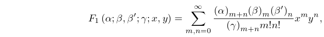
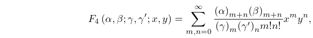
►The following four functions of two real or complex variables $x$ and $y$ cannot be expressed as a product of two ${}_2{}^{}F_1^{}$ functions, in general, but they satisfy partial differential equations that resemble the hypergeometric differential equation (15.10.1): ►

16.13.1 $$F_1(\alpha ;\beta ,{\beta }^{\prime };\gamma ;x,y)=\sum _{m,n=0}^{\mathrm{\infty }}\frac{{\left(\alpha \right)}_{m+n}{\left(\beta \right)}_m{\left({\beta }^{\prime }\right)}_n}{{\left(\gamma \right)}_{m+n}m!n!}{x}^m{y}^n,$$ ,

ⓘ

Defines:

$F_1(\alpha ;\beta ,{\beta }^{\prime };\gamma ;x,y)$: first Appell function

Symbols:

${\left(a\right)}_n$: Pochhammer’s symbol (or shifted factorial) and $!$: factorial (as in $n!$)

Permalink:

http://dlmf.nist.gov/16.13.E1

Encodings:

pMML, png, TeX

See also:

Annotations for §16.13 and Ch.16

… ►

16.13.4 $$F_4(\alpha ,\beta ;\gamma ,{\gamma }^{\prime };x,y)=\sum _{m,n=0}^{\mathrm{\infty }}\frac{{\left(\alpha \right)}_{m+n}{\left(\beta \right)}_{m+n}}{{\left(\gamma \right)}_m{\left({\gamma }^{\prime }\right)}_{n}m!n!}{x}^m{y}^n,$$ .

ⓘ

Defines:

$F_4(\alpha ,\beta ;\gamma ,{\gamma }^{\prime };x,y)$: fourth Appell function

Symbols:

${\left(a\right)}_n$: Pochhammer’s symbol (or shifted factorial) and $!$: factorial (as in $n!$)

Permalink:

http://dlmf.nist.gov/16.13.E4

Encodings:

pMML, png, TeX

See also:

Annotations for §16.13 and Ch.16

… ► …

14: 9.1 Special Notation

… ►(For other notation see Notation for the Special Functions.) ► ►►

$k$	nonnegative integer, except in §9.9(iii).
…

►The main functions treated in this chapter are the Airy functions $\mathrm{Ai}\left(z\right)$ and $\mathrm{Bi}\left(z\right)$, and the Scorer functions $\mathrm{Gi}(z)$ and $\mathrm{Hi}(z)$ (also known as inhomogeneous Airy functions). ►Other notations that have been used are as follows: $\mathrm{Ai}\left(-x\right)$ and $\mathrm{Bi}\left(-x\right)$ for $\mathrm{Ai}\left(x\right)$ and $\mathrm{Bi}\left(x\right)$ (Jeffreys (1928), later changed to $\mathrm{Ai}\left(x\right)$ and $\mathrm{Bi}\left(x\right)$); $U(x)=\sqrt{\pi }\mathrm{Bi}\left(x\right)$, $V(x)=\sqrt{\pi }\mathrm{Ai}\left(x\right)$ (Fock (1945)); $A(x)=3^{-1/3}\pi \mathrm{Ai}\left(-3^{-1/3}x\right)$ (Szegő (1967, §1.81)); $e_0(x)=\pi \mathrm{Hi}(-x)$, ${\tilde{e}}_0(x)=-\pi \mathrm{Gi}(-x)$ (Tumarkin (1959)).

15: 23.15 Definitions

§23.15 Definitions

►

§23.15(i) General Modular Functions

… ►If, as a function of $q$, $f(\tau )$ is analytic at $q=0$, then $f(\tau )$ is called a modular form. … ►

Dedekind’s Eta Function (or Dedekind Modular Function)

… ►

16: 14.20 Conical (or Mehler) Functions

… ► … ►Lastly, for the range , $P_{-\frac{1}{2}+\mathrm{i}\tau }^{-\mu }\left(x\right)$ is a real-valued solution of (14.20.1); in terms of $Q_{-\frac{1}{2}\pm \mathrm{i}\tau }^{\mu }\left(x\right)$ (which are complex-valued in general): … ►

§14.20(vi) Generalized Mehler–Fock Transformation

… ►

§14.20(viii) Asymptotic Approximations: Large $\tau$, $0\le \mu \le A\tau$

… ►

§14.20(ix) Asymptotic Approximations: Large $\mu$, $0\le \tau \le A\mu$

…

17: 11.9 Lommel Functions

§11.9 Lommel Functions

… ►can be regarded as a generalization of (11.2.7). Provided that $\mu \pm \nu \ne -1,-3,-5,\mathrm{\dots }$, (11.9.1) has the general solution … ► … ►

18: 20.2 Definitions and Periodic Properties

… ►

§20.2(i) Fourier Series

… ►

§20.2(ii) Periodicity and Quasi-Periodicity

… ►The four points $(0,\pi ,\pi +\tau \pi ,\tau \pi )$ are the vertices of the fundamental parallelogram in the $z$-plane; see Figure 20.2.1. …The theta functions are quasi-periodic on the lattice: … ►

§20.2(iv) $z$-Zeros

…

19: 9.12 Scorer Functions

§9.12 Scorer Functions

… ►The general solution is given by …where … ► … ►

Functions and Derivatives

…

20: 5.2 Definitions

… ►

§5.2(i) Gamma and Psi Functions

►

Euler’s Integral

►

5.2.1 $$\mathrm{\Gamma }\left(z\right)={\int }_0^{\mathrm{\infty }}{\mathrm{e}}^{-t}{t}^{z-1}dt,$$ $\mathrm{\Re }z>0$.

ⓘ

Defines:

$\mathrm{\Gamma }\left(z\right)$: gamma function

Symbols:

$dx$: differential of $x$ , $\mathrm{e}$: base of natural logarithm, $\int$: integral, $\mathrm{\Re }$: real part and $z$: complex variable

A&S Ref:

6.1.1

Referenced by:

§10.43(iii), (25.11.27), (25.11.28), (25.5.6), (25.5.7), §5.9(i), §5.9(ii), §8.21(ii), (9.12.17)

Permalink:

http://dlmf.nist.gov/5.2.E1

Encodings:

pMML, png, TeX

See also:

Annotations for §5.2(i), §5.2(i), §5.2 and Ch.5

►When $\mathrm{\Re }z\le 0$, $\mathrm{\Gamma }\left(z\right)$ is defined by analytic continuation. It is a meromorphic function with no zeros, and with simple poles of residue ${(-1)}^n/n!$ at $z=-n$. …