for modified Bessel functions

SearchAdvancedHelp

(0.024 seconds)

11—20 of 118 matching pages

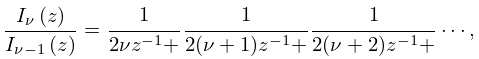
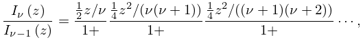
11: 10.33 Continued Fractions

§10.33 Continued Fractions

… ►

10.33.1 $$\frac{I_{\nu }\left(z\right)}{I_{\nu -1}\left(z\right)}=\frac{1}{2\nu z^{-1}+}\frac{1}{2(\nu +1)z^{-1}+}\frac{1}{2(\nu +2)z^{-1}+}\mathrm{\cdots },$$ $z\ne 0$,

ⓘ

Symbols:

$I_{\nu }\left(z\right)$: modified Bessel function of the first kind, $z$: complex variable and $\nu$: complex parameter

Referenced by:

§10.74(v)

Permalink:

http://dlmf.nist.gov/10.33.E1

Encodings:

pMML, png, TeX

See also:

Annotations for §10.33 and Ch.10

►

10.33.2 $$\frac{I_{\nu }\left(z\right)}{I_{\nu -1}\left(z\right)}=\frac{\frac{1}{2}z/\nu }{1+}\frac{\frac{1}{4}{z}^2/(\nu (\nu +1))}{1+}\frac{\frac{1}{4}{z}^2/((\nu +1)(\nu +2))}{1+}\mathrm{\cdots },$$ $\nu \ne 0,-1,-2,\mathrm{\dots }$.

ⓘ

Symbols:

$I_{\nu }\left(z\right)$: modified Bessel function of the first kind, $z$: complex variable and $\nu$: complex parameter

Referenced by:

§10.74(v)

Permalink:

http://dlmf.nist.gov/10.33.E2

Encodings:

pMML, png, TeX

See also:

Annotations for §10.33 and Ch.10

…

12: 10.72 Mathematical Applications

… ►

§10.72(i) Differential Equations with Turning Points

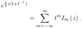
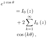
►Bessel functions and modified Bessel functions are often used as approximants in the construction of uniform asymptotic approximations and expansions for solutions of linear second-order differential equations containing a parameter. … ►If $f(z)$ has a double zero $z_0$, or more generally $z_0$ is a zero of order $m$, $m=2,3,4,\mathrm{\dots }$, then uniform asymptotic approximations (but not expansions) can be constructed in terms of Bessel functions, or modified Bessel functions, of order $1/(m+2)$. …The order of the approximating Bessel functions, or modified Bessel functions, is $1/(\lambda +2)$, except in the case when $g(z)$ has a double pole at $z_0$. … ►Then for large $u$ asymptotic approximations of the solutions $w$ can be constructed in terms of Bessel functions, or modified Bessel functions, of variable order (in fact the order depends on $u$ and $\alpha$). …

13: 10.35 Generating Function and Associated Series

§10.35 Generating Function and Associated Series

… ►

10.35.1 $${\mathrm{e}}^{\frac{1}{2}z(t+t^{-1})}=\sum _{m=-\mathrm{\infty }}^{\mathrm{\infty }}{t}^m{I}_m\left(z\right).$$

ⓘ

Symbols:

$\mathrm{e}$: base of natural logarithm, $I_{\nu }\left(z\right)$: modified Bessel function of the first kind, $m$: integer and $z$: complex variable

A&S Ref:

9.6.33

Referenced by:

§10.35

Permalink:

http://dlmf.nist.gov/10.35.E1

Encodings:

pMML, png, TeX

See also:

Annotations for §10.35 and Ch.10

… ►

10.35.2 $${\mathrm{e}}^{z\cos \theta }=I_0\left(z\right)+2\sum _{k=1}^{\mathrm{\infty }}{I}_k\left(z\right)\cos \left(k\theta \right),$$

ⓘ

Symbols:

$\cos z$: cosine function, $\mathrm{e}$: base of natural logarithm, $I_{\nu }\left(z\right)$: modified Bessel function of the first kind, $k$: nonnegative integer and $z$: complex variable

A&S Ref:

9.6.34

Referenced by:

§10.35

Permalink:

http://dlmf.nist.gov/10.35.E2

Encodings:

pMML, png, TeX

See also:

Annotations for §10.35 and Ch.10

… ►

10.35.4 $$1=I_0\left(z\right)-2I_2\left(z\right)+2I_4\left(z\right)-2I_6\left(z\right)+\mathrm{\cdots },$$

ⓘ

Symbols:

$I_{\nu }\left(z\right)$: modified Bessel function of the first kind and $z$: complex variable

A&S Ref:

9.6.36

Permalink:

http://dlmf.nist.gov/10.35.E4

Encodings:

pMML, png, TeX

See also:

Annotations for §10.35 and Ch.10

►

10.35.5 $${\mathrm{e}}^{\pm z}=I_0\left(z\right)\pm 2I_1\left(z\right)+2I_2\left(z\right)\pm 2I_3\left(z\right)+\mathrm{\cdots },$$

ⓘ

Symbols:

$\mathrm{e}$: base of natural logarithm, $I_{\nu }\left(z\right)$: modified Bessel function of the first kind and $z$: complex variable

A&S Ref:

9.6.37,9.6.38

Permalink:

http://dlmf.nist.gov/10.35.E5

Encodings:

pMML, png, TeX

See also:

Annotations for §10.35 and Ch.10

…

14: 10.46 Generalized and Incomplete Bessel Functions; Mittag-Leffler Function

… ►

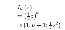
10.46.2 $$I_{\nu }\left(z\right)={\left(\frac{1}{2}z\right)}^{\nu }\varphi (1,\nu +1;\frac{1}{4}{z}^2).$$

ⓘ

Symbols:

$\varphi (\rho ,\beta ;z)$: generalized Bessel function, $I_{\nu }\left(z\right)$: modified Bessel function of the first kind, $z$: complex variable and $\nu$: complex parameter

Permalink:

http://dlmf.nist.gov/10.46.E2

Encodings:

pMML, png, TeX

See also:

Annotations for §10.46 and Ch.10

… ►For incomplete modified Bessel functions and Hankel functions, including applications, see Cicchetti and Faraone (2004).

15: 10.25 Definitions

… ►Its solutions are called modified Bessel functions or Bessel functions of imaginary argument. ►

§10.25(ii) Standard Solutions

… ►

Branch Conventions

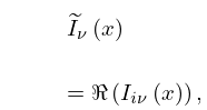
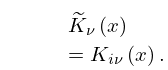
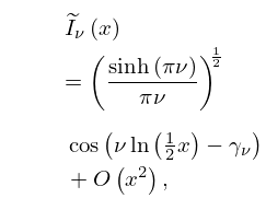
… ►Corresponding to the symbol ${𝒞}_{\nu }$ introduced in §10.2(ii), we sometimes use ${𝒵}_{\nu }\left(z\right)$ to denote $I_{\nu }\left(z\right)$, ${\mathrm{e}}^{\nu \pi \mathrm{i}}{K}_{\nu }\left(z\right)$, or any nontrivial linear combination of these functions, the coefficients in which are independent of $z$ and $\nu$. …

16: 10.45 Functions of Imaginary Order

§10.45 Functions of Imaginary Order

… ►

10.45.2 ${\tilde{I}}_{\nu }\left(x\right)=\mathrm{\Re }\left(I_{\mathrm{i}\nu }\left(x\right)\right),$ ${\tilde{K}}_{\nu }\left(x\right)=K_{\mathrm{i}\nu }\left(x\right).$

ⓘ

Defines:

${\tilde{I}}_{\nu }\left(x\right)$: modified Bessel function of the first kind of imaginary order and ${\tilde{K}}_{\nu }\left(x\right)$: modified Bessel function fo the second kind of imaginary order

Symbols:

$\mathrm{i}$: imaginary unit, $I_{\nu }\left(z\right)$: modified Bessel function of the first kind, $K_{\nu }\left(z\right)$: modified Bessel function of the second kind, $\mathrm{\Re }$: real part, $x$: real variable and $\nu$: complex parameter

Referenced by:

§10.30(i), §10.74(viii)

Permalink:

http://dlmf.nist.gov/10.45.E2

Encodings:

pMML, pMML, png, png, TeX, TeX

See also:

Annotations for §10.45 and Ch.10

… ►

10.45.6 $${\tilde{I}}_{\nu }\left(x\right)={\left(\frac{\sinh \left(\pi \nu \right)}{\pi \nu }\right)}^{\frac{1}{2}}\cos \left(\nu \ln \left(\frac{1}{2}x\right)-{\gamma }_{\nu }\right)+O\left(x^2\right),$$

ⓘ

Symbols:

$O\left(x\right)$: order not exceeding, $\pi$: the ratio of the circumference of a circle to its diameter, $\cos z$: cosine function, $\sinh z$: hyperbolic sine function, ${\tilde{I}}_{\nu }\left(x\right)$: modified Bessel function of the first kind of imaginary order, $\ln z$: principal branch of logarithm function, $x$: real variable, $\nu$: complex parameter and ${\gamma }_{\nu }$: parameter

Referenced by:

§10.45

Permalink:

http://dlmf.nist.gov/10.45.E6

Encodings:

pMML, png, TeX

See also:

Annotations for §10.45 and Ch.10

… ► … ►

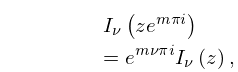
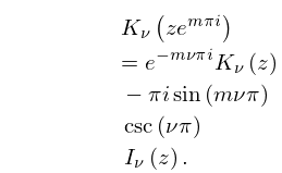
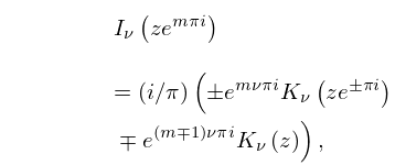
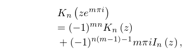
17: 10.34 Analytic Continuation

§10.34 Analytic Continuation

… ►

10.34.1 $$I_{\nu }\left(z{\mathrm{e}}^{m\pi \mathrm{i}}\right)={\mathrm{e}}^{m\nu \pi \mathrm{i}}{I}_{\nu }\left(z\right),$$

ⓘ

Symbols:

$\pi$: the ratio of the circumference of a circle to its diameter, $\mathrm{e}$: base of natural logarithm, $\mathrm{i}$: imaginary unit, $I_{\nu }\left(z\right)$: modified Bessel function of the first kind, $m$: integer, $z$: complex variable and $\nu$: complex parameter

A&S Ref:

9.6.30

Referenced by:

§10.30(ii), §10.34, §10.47(v)

Permalink:

http://dlmf.nist.gov/10.34.E1

Encodings:

pMML, png, TeX

See also:

Annotations for §10.34 and Ch.10

►

10.34.2 $$K_{\nu }\left(z{\mathrm{e}}^{m\pi \mathrm{i}}\right)={\mathrm{e}}^{-m\nu \pi \mathrm{i}}{K}_{\nu }\left(z\right)-\pi \mathrm{i}\sin \left(m\nu \pi \right)\csc \left(\nu \pi \right)I_{\nu }\left(z\right).$$

ⓘ

Symbols:

$\pi$: the ratio of the circumference of a circle to its diameter, $\csc z$: cosecant function, $\mathrm{e}$: base of natural logarithm, $\mathrm{i}$: imaginary unit, $I_{\nu }\left(z\right)$: modified Bessel function of the first kind, $K_{\nu }\left(z\right)$: modified Bessel function of the second kind, $\sin z$: sine function, $m$: integer, $z$: complex variable and $\nu$: complex parameter

A&S Ref:

9.6.31

Referenced by:

§10.27, §10.34, §10.34

Permalink:

http://dlmf.nist.gov/10.34.E2

Encodings:

pMML, png, TeX

See also:

Annotations for §10.34 and Ch.10

►

10.34.3 $$I_{\nu }\left(z{\mathrm{e}}^{m\pi \mathrm{i}}\right)=(\mathrm{i}/\pi )\left(\pm {\mathrm{e}}^{m\nu \pi \mathrm{i}}{K}_{\nu }\left(z{\mathrm{e}}^{\pm \pi \mathrm{i}}\right)\mp {\mathrm{e}}^{(m\mp 1)\nu \pi \mathrm{i}}{K}_{\nu }\left(z\right)\right),$$

ⓘ

Symbols:

$\pi$: the ratio of the circumference of a circle to its diameter, $\mathrm{e}$: base of natural logarithm, $\mathrm{i}$: imaginary unit, $I_{\nu }\left(z\right)$: modified Bessel function of the first kind, $K_{\nu }\left(z\right)$: modified Bessel function of the second kind, $m$: integer, $z$: complex variable and $\nu$: complex parameter

Referenced by:

§10.34, §10.40(i), §10.40(iii), §10.41(iv)

Permalink:

http://dlmf.nist.gov/10.34.E3

Encodings:

pMML, png, TeX

See also:

Annotations for §10.34 and Ch.10

… ►

10.34.5 $$K_n\left(z{\mathrm{e}}^{m\pi \mathrm{i}}\right)={(-1)}^{mn}{K}_n\left(z\right)+{(-1)}^{n(m-1)-1}m\pi \mathrm{i}{I}_n\left(z\right),$$

ⓘ

Symbols:

$\pi$: the ratio of the circumference of a circle to its diameter, $\mathrm{e}$: base of natural logarithm, $\mathrm{i}$: imaginary unit, $I_{\nu }\left(z\right)$: modified Bessel function of the first kind, $K_{\nu }\left(z\right)$: modified Bessel function of the second kind, $m$: integer, $n$: integer and $z$: complex variable

Permalink:

http://dlmf.nist.gov/10.34.E5

Encodings:

pMML, png, TeX

See also:

Annotations for §10.34 and Ch.10

…

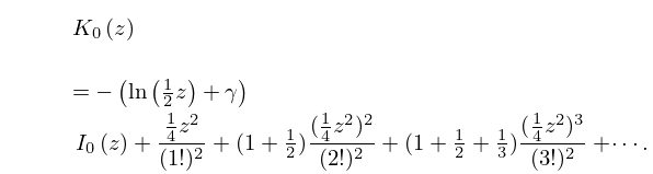
18: 10.31 Power Series

§10.31 Power Series

… ►

10.31.1 $$K_n\left(z\right)=\frac{1}{2}{(\frac{1}{2}z)}^{-n}\sum _{k=0}^{n-1}\frac{(n-k-1)!}{k!}{(-\frac{1}{4}{z}^2)}^k+{(-1)}^{n+1}\ln \left(\frac{1}{2}z\right)I_n\left(z\right)+{(-1)}^n\frac{1}{2}{(\frac{1}{2}z)}^n\sum _{k=0}^{\mathrm{\infty }}\left(\psi \left(k+1\right)+\psi \left(n+k+1\right)\right)\frac{{(\frac{1}{4}{z}^2)}^k}{k!(n+k)!},$$

ⓘ

Symbols:

$\psi \left(z\right)$: psi (or digamma) function, $!$: factorial (as in $n!$), $I_{\nu }\left(z\right)$: modified Bessel function of the first kind, $K_{\nu }\left(z\right)$: modified Bessel function of the second kind, $\ln z$: principal branch of logarithm function, $n$: integer, $k$: nonnegative integer and $z$: complex variable

A&S Ref:

9.6.11

Referenced by:

§10.30(i), §10.65(ii)

Permalink:

http://dlmf.nist.gov/10.31.E1

Encodings:

pMML, png, TeX

See also:

Annotations for §10.31 and Ch.10

… ►

10.31.2 $$K_0\left(z\right)=-\left(\ln \left(\frac{1}{2}z\right)+\gamma \right)I_0\left(z\right)+\frac{\frac{1}{4}{z}^2}{{(1!)}^2}+(1+\frac{1}{2})\frac{{(\frac{1}{4}{z}^2)}^2}{{(2!)}^2}+(1+\frac{1}{2}+\frac{1}{3})\frac{{(\frac{1}{4}{z}^2)}^3}{{(3!)}^2}+\mathrm{\cdots }.$$

ⓘ

Symbols:

$\gamma$: Euler’s constant, $!$: factorial (as in $n!$), $I_{\nu }\left(z\right)$: modified Bessel function of the first kind, $K_{\nu }\left(z\right)$: modified Bessel function of the second kind, $\ln z$: principal branch of logarithm function and $z$: complex variable

A&S Ref:

9.6.13

Referenced by:

§10.45

Permalink:

http://dlmf.nist.gov/10.31.E2

Encodings:

pMML, png, TeX

See also:

Annotations for §10.31 and Ch.10

… ►

10.31.3 $$I_{\nu }\left(z\right)I_{\mu }\left(z\right)={(\frac{1}{2}z)}^{\nu +\mu }\sum _{k=0}^{\mathrm{\infty }}\frac{{\left(\nu +\mu +k+1\right)}_k{(\frac{1}{4}{z}^2)}^k}{k!\mathrm{\Gamma }\left(\nu +k+1\right)\mathrm{\Gamma }\left(\mu +k+1\right)}.$$

ⓘ

Symbols:

$\mathrm{\Gamma }\left(z\right)$: gamma function, ${\left(a\right)}_n$: Pochhammer’s symbol (or shifted factorial), $!$: factorial (as in $n!$), $I_{\nu }\left(z\right)$: modified Bessel function of the first kind, $k$: nonnegative integer, $z$: complex variable and $\nu$: complex parameter

Referenced by:

§10.31

Permalink:

http://dlmf.nist.gov/10.31.E3

Encodings:

pMML, png, TeX

Correction (effective with 1.1.2):

The Pochhammer symbol now links to its definition.

See also:

Annotations for §10.31 and Ch.10

19: 10.66 Expansions in Series of Bessel Functions

… ►

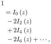
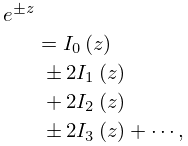
10.66.1 $${\mathrm{ber}}_{\nu }x+\mathrm{i}{\mathrm{bei}}_{\nu }x=\sum _{k=0}^{\mathrm{\infty }}\frac{{\mathrm{e}}^{(3\nu +k)\pi \mathrm{i}/4}{x}^k{J}_{\nu +k}\left(x\right)}{2^{k/2}k!}=\sum _{k=0}^{\mathrm{\infty }}\frac{{\mathrm{e}}^{(3\nu +3k)\pi \mathrm{i}/4}{x}^k{I}_{\nu +k}\left(x\right)}{2^{k/2}k!}.$$

ⓘ

Symbols:

$J_{\nu }\left(z\right)$: Bessel function of the first kind, ${\mathrm{bei}}_{\nu }\left(x\right)$: Kelvin function, ${\mathrm{ber}}_{\nu }\left(x\right)$: Kelvin function, $\pi$: the ratio of the circumference of a circle to its diameter, $\mathrm{e}$: base of natural logarithm, $!$: factorial (as in $n!$), $\mathrm{i}$: imaginary unit, $I_{\nu }\left(z\right)$: modified Bessel function of the first kind, $k$: nonnegative integer, $x$: real variable and $\nu$: complex parameter

A&S Ref:

9.9.32

Referenced by:

§10.66

Permalink:

http://dlmf.nist.gov/10.66.E1

Encodings:

pMML, png, TeX

See also:

Annotations for §10.66 and Ch.10

…

20: 10.40 Asymptotic Expansions for Large Argument

§10.40 Asymptotic Expansions for Large Argument

►

§10.40(i) Hankel’s Expansions

… ►

Products

… ► … ►

§10.40(iv) Exponentially-Improved Expansions

…