…
►The functions treated in this chapter are the three principal Jacobian ellipticfunctions
, , ; the nine subsidiary Jacobian ellipticfunctions
, , , , , , , , ; the amplitude function
; Jacobi’s epsilon and zeta functions
and .
►The notation , , is due to Gudermann (1838), following Jacobi (1827); that for the subsidiary functions is due to Glaisher (1882).
Other notations for are and with ; see Abramowitz and Stegun (1964) and Walker (1996).
…
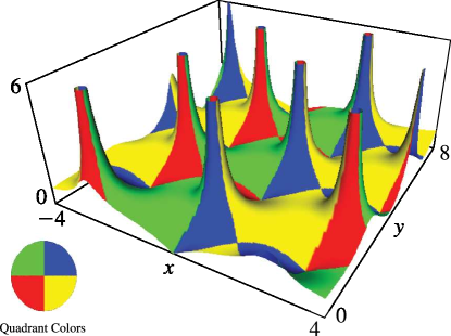
►Figure 22.3.25:
as a function of complex , , .
…
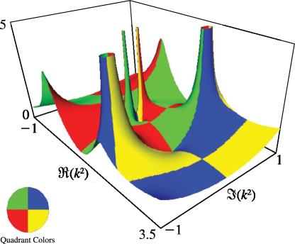
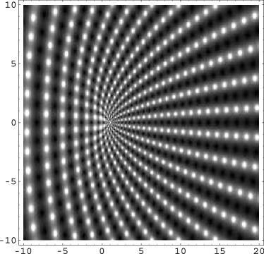
Magnify3DHelp►►►Figure 22.3.26: Density plot of as a function of complex , , .
…
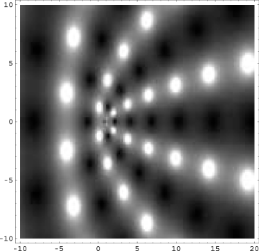
Magnify►►►Figure 22.3.27: Density plot of as a function of complex , , .
…
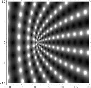
Magnify►►►Figure 22.3.28: Density plot of as a function of complex , , .
…
Magnify
…
►The main functions treated in this chapter are the Weierstrass -function
; the Weierstrass zeta function
; the Weierstrass sigma function
; the elliptic modular function
; Klein’s complete invariant ; Dedekind’s eta function
.
…
…
►In §22.19(ii) it is noted that Jacobian ellipticfunctions provide a natural basis of solutions for problems in Newtonian classical dynamics with quartic potentials in canonical form .
…
►
 ►
►
 ►
►
 ►
►
 ►
►
 ►
►
