for confluent hypergeometric functions
(0.021 seconds)
11—20 of 95 matching pages
11: 13.1 Special Notation
…
►The main functions treated in this chapter are the Kummer functions
and , Olver’s function
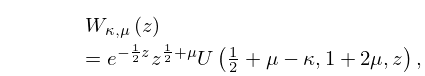
, and the Whittaker functions
and .
…
►
12: 13.10 Integrals
13: 13.14 Definitions and Basic Properties
…
►
13.14.3
…
►Except when , each branch of the functions
and is entire in and .
…
►
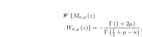
13.14.26
…
►
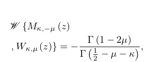
13.14.28
…
►
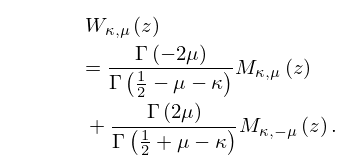
13.14.33
14: 13.23 Integrals
…
►
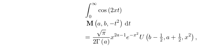
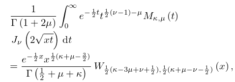
13.23.10
, .
…
►
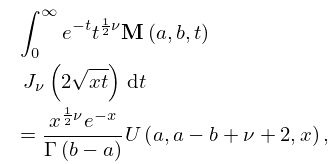
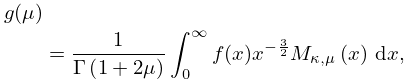
13.23.12
, .
…
►
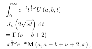
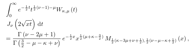
13.23.13
►
13.23.14
…
►Additional integrals involving confluent hypergeometric functions can be found in Apelblat (1983, pp. 388–392), Erdélyi et al. (1954b), Gradshteyn and Ryzhik (2000, §7.6), and Prudnikov et al. (1990, §§1.13, 1.14, 2.19, 4.2.2).
…
15: 10.16 Relations to Other Functions
…
►
Confluent Hypergeometric Functions
►
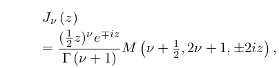
10.16.5
…
►For the functions
and see §13.2(i).
►
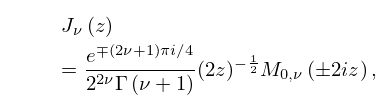
10.16.7
,
…
►For the functions
and see §13.14(i).
…
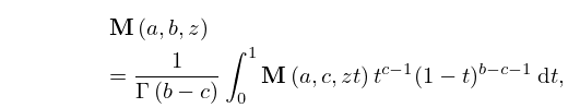
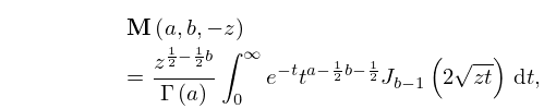
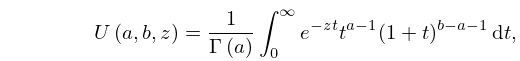
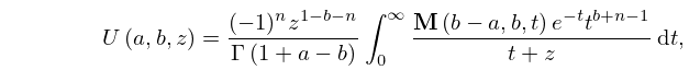
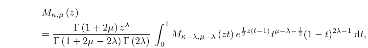
16: 13.4 Integral Representations
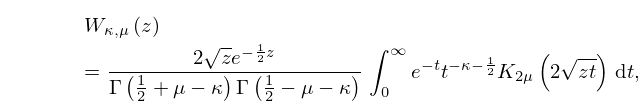
17: 13.16 Integral Representations
18: 12.18 Methods of Computation
…
►Because PCFs are special cases of confluent hypergeometric functions, the methods of computation described in §13.29 are applicable to PCFs.
…
19: 10.39 Relations to Other Functions
…
►
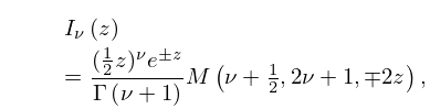
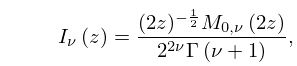
Confluent Hypergeometric Functions
►
10.39.5
…
►
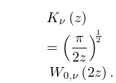
10.39.7
,
►
10.39.8
►For the functions
, , , and see §§13.2(i) and 13.14(i).
…
