About the Project

for%20large%20%7C%CE%B32%7C

AdvancedHelp

Did you mean for%20large%20%7C%CE%132%7C ?

(0.004 seconds)

1—10 of 410 matching pages

1: 28.16 Asymptotic Expansions for Large q
§28.16 Asymptotic Expansions for Large q
28.16.1 λ ν ( h 2 ) 2 h 2 + 2 s h 1 8 ( s 2 + 1 ) 1 2 7 h ( s 3 + 3 s ) 1 2 12 h 2 ( 5 s 4 + 34 s 2 + 9 ) 1 2 17 h 3 ( 33 s 5 + 410 s 3 + 405 s ) 1 2 20 h 4 ( 63 s 6 + 1260 s 4 + 2943 s 2 + 486 ) 1 2 25 h 5 ( 527 s 7 + 15617 s 5 + 69001 s 3 + 41607 s ) + .
2: 20 Theta Functions
Chapter 20 Theta Functions
3: Staff
  • Ronald F. Boisvert, Editor at Large, NIST

  • William P. Reinhardt, University of Washington, Chaps. 20, 22, 23

  • Peter L. Walker, American University of Sharjah, Chaps. 20, 22, 23

  • William P. Reinhardt, University of Washington, for Chaps. 20, 22, 23

  • Peter L. Walker, American University of Sharjah, for Chaps. 20, 22, 23

  • 4: 19.2 Definitions
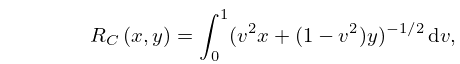
    §19.2(iv) A Related Function: R C ( x , y )
    Formulas involving Π ( ϕ , α 2 , k ) that are customarily different for circular cases, ordinary hyperbolic cases, and (hyperbolic) Cauchy principal values, are united in a single formula by using R C ( x , y ) . … When x and y are positive, R C ( x , y ) is an inverse circular function if x < y and an inverse hyperbolic function (or logarithm) if x > y : …For the special cases of R C ( x , x ) and R C ( 0 , y ) see (19.6.15). …
    19.2.21 R C ( x , y ) = 0 1 ( v 2 x + ( 1 v 2 ) y ) 1 / 2 d v ,
    5: 23 Weierstrass Elliptic and Modular
    Functions
    6: 3.4 Differentiation
    B 2 5 = 1 120 ( 6 10 t 15 t 2 + 20 t 3 5 t 4 ) ,
    B 3 7 = 1 720 ( 48 + 8 t 192 t 2 20 t 3 + 85 t 4 + 6 t 5 7 t 6 ) ,
    where C is a simple closed contour described in the positive rotational sense such that C and its interior lie in the domain of analyticity of f , and x 0 is interior to C . Taking C to be a circle of radius r centered at x 0 , we obtain … With the choice r = k (which is crucial when k is large because of numerical cancellation) the integrand equals e k at the dominant points θ = 0 , 2 π , and in combination with the factor k k in front of the integral sign this gives a rough approximation to 1 / k ! . …
    7: 28.35 Tables
  • Blanch and Clemm (1965) includes values of Mc n ( 2 ) ( x , q ) , Mc n ( 2 ) ( x , q ) for n = 0 ( 1 ) 7 , x = 0 ( .02 ) 1 ; n = 8 ( 1 ) 15 , x = 0 ( .01 ) 1 . Also Ms n ( 2 ) ( x , q ) , Ms n ( 2 ) ( x , q ) for n = 1 ( 1 ) 7 , x = 0 ( .02 ) 1 ; n = 8 ( 1 ) 15 , x = 0 ( .01 ) 1 . In all cases q = 0 ( .05 ) 1 . Precision is generally 7D. Approximate formulas and graphs are also included.

  • Ince (1932) includes eigenvalues a n , b n , and Fourier coefficients for n = 0 or 1 ( 1 ) 6 , q = 0 ( 1 ) 10 ( 2 ) 20 ( 4 ) 40 ; 7D. Also ce n ( x , q ) , se n ( x , q ) for q = 0 ( 1 ) 10 , x = 1 ( 1 ) 90 , corresponding to the eigenvalues in the tables; 5D. Notation: a n = 𝑏𝑒 n 2 q , b n = 𝑏𝑜 n 2 q .

  • Kirkpatrick (1960) contains tables of the modified functions Ce n ( x , q ) , Se n + 1 ( x , q ) for n = 0 ( 1 ) 5 , q = 1 ( 1 ) 20 , x = 0.1 ( .1 ) 1 ; 4D or 5D.

  • National Bureau of Standards (1967) includes the eigenvalues a n ( q ) , b n ( q ) for n = 0 ( 1 ) 3 with q = 0 ( .2 ) 20 ( .5 ) 37 ( 1 ) 100 , and n = 4 ( 1 ) 15 with q = 0 ( 2 ) 100 ; Fourier coefficients for ce n ( x , q ) and se n ( x , q ) for n = 0 ( 1 ) 15 , n = 1 ( 1 ) 15 , respectively, and various values of q in the interval [ 0 , 100 ] ; joining factors g e , n ( q ) , f e , n ( q ) for n = 0 ( 1 ) 15 with q = 0 ( .5  to  10 ) 100 (but in a different notation). Also, eigenvalues for large values of q . Precision is generally 8D.

  • Zhang and Jin (1996, pp. 521–532) includes the eigenvalues a n ( q ) , b n + 1 ( q ) for n = 0 ( 1 ) 4 , q = 0 ( 1 ) 50 ; n = 0 ( 1 ) 20 ( a ’s) or 19 ( b ’s), q = 1 , 3 , 5 , 10 , 15 , 25 , 50 ( 50 ) 200 . Fourier coefficients for ce n ( x , 10 ) , se n + 1 ( x , 10 ) , n = 0 ( 1 ) 7 . Mathieu functions ce n ( x , 10 ) , se n + 1 ( x , 10 ) , and their first x -derivatives for n = 0 ( 1 ) 4 , x = 0 ( 5 ) 90 . Modified Mathieu functions Mc n ( j ) ( x , 10 ) , Ms n + 1 ( j ) ( x , 10 ) , and their first x -derivatives for n = 0 ( 1 ) 4 , j = 1 , 2 , x = 0 ( .2 ) 4 . Precision is mostly 9S.

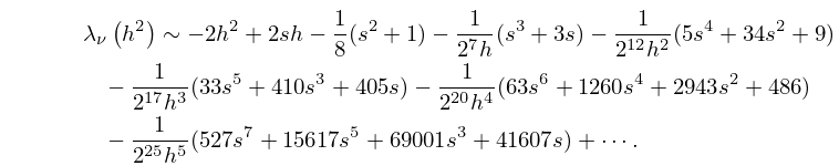
  • 8: 28.8 Asymptotic Expansions for Large q
    §28.8 Asymptotic Expansions for Large q
    §28.8(ii) Sips’ Expansions
    §28.8(iii) Goldstein’s Expansions
    Barrett’s Expansions
    9: 10.75 Tables
  • Achenbach (1986) tabulates J 0 ( x ) , J 1 ( x ) , Y 0 ( x ) , Y 1 ( x ) , x = 0 ( .1 ) 8 , 20D or 18–20S.

  • Bickley et al. (1952) tabulates x n I n ( x ) or e x I n ( x ) , x n K n ( x ) or e x K n ( x ) , n = 2 ( 1 ) 20 , x = 0 (.01 or .1) 10(.1) 20, 8S; I n ( x ) , K n ( x ) , n = 0 ( 1 ) 20 , x = 0 or 0.1 ( .1 ) 20 , 10S.

  • Kerimov and Skorokhodov (1984b) tabulates all zeros of the principal values of K n ( z ) and K n ( z ) , for n = 2 ( 1 ) 20 , 9S.

  • Zhang and Jin (1996, p. 322) tabulates ber x , ber x , bei x , bei x , ker x , ker x , kei x , kei x , x = 0 ( 1 ) 20 , 7S.

  • Zhang and Jin (1996, p. 323) tabulates the first 20 real zeros of ber x , ber x , bei x , bei x , ker x , ker x , kei x , kei x , 8D.

  • 10: 8.26 Tables
  • Khamis (1965) tabulates P ( a , x ) for a = 0.05 ( .05 ) 10 ( .1 ) 20 ( .25 ) 70 , 0.0001 x 250 to 10D.

  • Abramowitz and Stegun (1964, pp. 245–248) tabulates E n ( x ) for n = 2 , 3 , 4 , 10 , 20 , x = 0 ( .01 ) 2 to 7D; also ( x + n ) e x E n ( x ) for n = 2 , 3 , 4 , 10 , 20 , x 1 = 0 ( .01 ) 0.1 ( .05 ) 0.5 to 6S.

  • Pagurova (1961) tabulates E n ( x ) for n = 0 ( 1 ) 20 , x = 0 ( .01 ) 2 ( .1 ) 10 to 4-9S; e x E n ( x ) for n = 2 ( 1 ) 10 , x = 10 ( .1 ) 20 to 7D; e x E p ( x ) for p = 0 ( .1 ) 1 , x = 0.01 ( .01 ) 7 ( .05 ) 12 ( .1 ) 20 to 7S or 7D.

  • Zhang and Jin (1996, Table 19.1) tabulates E n ( x ) for n = 1 , 2 , 3 , 5 , 10 , 15 , 20 , x = 0 ( .1 ) 1 , 1.5 , 2 , 3 , 5 , 10 , 20 , 30 , 50 , 100 to 7D or 8S.