for%20derivatives

SearchAdvancedHelp

(0.002 seconds)

1—10 of 33 matching pages

1: 9.18 Tables

… ►

Miller (1946) tabulates $a_k$, ${\mathrm{Ai}}^{\prime }\left(a_k\right)$, $a_k^{\prime }$, $\mathrm{Ai}\left(a_k^{\prime }\right)$, $k=1(1)50$; $b_k$, ${\mathrm{Bi}}^{\prime }\left(b_k\right)$, $b_k^{\prime }$, $\mathrm{Bi}\left(b_k^{\prime }\right)$, $k=1(1)20$. Precision is 8D. Entries for $k=1(1)20$ are reproduced in Abramowitz and Stegun (1964, Chapter 10).

►

Sherry (1959) tabulates $a_k$, ${\mathrm{Ai}}^{\prime }\left(a_k\right)$, $a_k^{\prime }$, $\mathrm{Ai}\left(a_k^{\prime }\right)$, $k=1(1)50$; 20S.

►

Zhang and Jin (1996, p. 339) tabulates $a_k$, ${\mathrm{Ai}}^{\prime }\left(a_k\right)$, $a_k^{\prime }$, $\mathrm{Ai}\left(a_k^{\prime }\right)$, $b_k$, ${\mathrm{Bi}}^{\prime }\left(b_k\right)$, $b_k^{\prime }$, $\mathrm{Bi}\left(b_k^{\prime }\right)$, $k=1(1)20$; 8D.

…

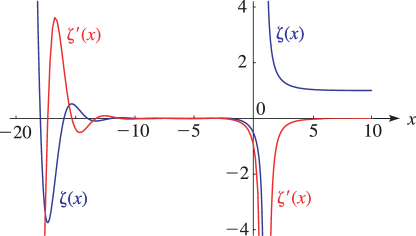
2: 25.3 Graphics

… ►

►►

Figure 25.3.1: Riemann zeta function $\zeta \left(x\right)$ and its derivative ${\zeta }^{\prime }\left(x\right)$, $-20\le x\le 10$. Magnify

…

3: 10.75 Tables

… ►

Olver (1960) tabulates $j_{n,m}$, $J_n^{\prime }\left(j_{n,m}\right)$, $j_{n,m}^{\prime }$, $J_n\left(j_{n,m}^{\prime }\right)$, $y_{n,m}$, $Y_n^{\prime }\left(y_{n,m}\right)$, $y_{n,m}^{\prime }$, $Y_n\left(y_{n,m}^{\prime }\right)$, $n=0(\frac{1}{2})20⁤\frac{1}{2}$, $m=1(1)50$, 8D. Also included are tables of the coefficients in the uniform asymptotic expansions of these zeros and associated values as $n\to \mathrm{\infty }$; see §10.21(viii), and more fully Olver (1954).

… ►

Abramowitz and Stegun (1964, Chapter 9) tabulates $j_{n,m}$, $J_n^{\prime }\left(j_{n,m}\right)$, $j_{n,m}^{\prime }$, $J_n\left(j_{n,m}^{\prime }\right)$, $n=0(1)8$, $m=1(1)20$, 5D (10D for $n=0$), $y_{n,m}$, $Y_n^{\prime }\left(y_{n,m}\right)$, $y_{n,m}^{\prime }$, $Y_n\left(y_{n,m}^{\prime }\right)$, $n=0(1)8$, $m=1(1)20$, 5D (8D for $n=0$), $J_0\left(j_{0,m}x\right)$, $m=1(1)5$, $x=0(.02)1$, 5D. Also included are the first 5 zeros of the functions $x{J}_1\left(x\right)-\lambda J_0\left(x\right)$, $J_1\left(x\right)-\lambda x{J}_0\left(x\right)$, $J_0\left(x\right)Y_0\left(\lambda x\right)-Y_0\left(x\right)J_0\left(\lambda x\right)$, $J_1\left(x\right)Y_1\left(\lambda x\right)-Y_1\left(x\right)J_1\left(\lambda x\right)$, $J_1\left(x\right)Y_0\left(\lambda x\right)-Y_1\left(x\right)J_0\left(\lambda x\right)$ for various values of $\lambda$ and ${\lambda }^{-1}$ in the interval $[0,1]$, 4–8D.

… ►

Zhang and Jin (1996, pp. 296–305) tabulates ${𝗃}_n\left(x\right)$, ${𝗃}_n^{\prime }\left(x\right)$, ${𝗒}_n\left(x\right)$, ${𝗒}_n^{\prime }\left(x\right)$, ${𝗂}_n^{(1)}\left(x\right)$, $𝗂_n^{(1)}{}_{}{}^{\prime }\left(x\right)$, ${𝗄}_n\left(x\right)$, ${𝗄}_n^{\prime }\left(x\right)$, $n=0(1)10(10)30$, 50, 100, $x=1$, 5, 10, 25, 50, 100, 8S; $x{𝗃}_n\left(x\right)$, ${(x{𝗃}_n\left(x\right))}^{\prime }$, $x{𝗒}_n\left(x\right)$, ${(x{𝗒}_n\left(x\right))}^{\prime }$ (Riccati–Bessel functions and their derivatives), $n=0(1)10(10)30$, 50, 100, $x=1$, 5, 10, 25, 50, 100, 8S; real and imaginary parts of ${𝗃}_n\left(z\right)$, ${𝗃}_n^{\prime }\left(z\right)$, ${𝗒}_n\left(z\right)$, ${𝗒}_n^{\prime }\left(z\right)$, ${𝗂}_n^{(1)}\left(z\right)$, $𝗂_n^{(1)}{}_{}{}^{\prime }\left(z\right)$, ${𝗄}_n\left(z\right)$, ${𝗄}_n^{\prime }\left(z\right)$, $n=0(1)15$, 20(10)50, 100, $z=4+2\mathrm{i}$, $20+10\mathrm{i}$, 8S. (For the notation replace $j,y,\mathrm{i},k$ by $𝗃$, $𝗒$, ${𝗂}^{(1)}$, $𝗄$, respectively.)

…

4: 3.8 Nonlinear Equations

… ►

3.8.16 $$\frac{dx}{d{a}_{19}}=-\frac{{20}^{19}}{19!}=(-4.30\mathrm{\dots })\times {10}^7.$$

ⓘ

Symbols:

$\frac{df}{dx}$: derivative of $f$ with respect to $x$ and $!$: factorial (as in $n!$)

Permalink:

http://dlmf.nist.gov/3.8.E16

Encodings:

pMML, png, TeX

See also:

Annotations for §3.8(vi), §3.8(vi), §3.8 and Ch.3

…

5: Bibliography

… ►

Repeated integrals and derivatives of $K$ Bessel functions. SIAM J. Math. Anal. 20 (1), pp. 169–175.

ⓘ

External Links:

ISSN 0036-1410, Document, MathReview (A. Haimovici), ZentralBlatt

Referenced by:

§10.43(iii).

Encodings:

BibTeX

…

6: 9.9 Zeros

… ►

9.9.8 $$a_k^{\prime }=-U\left(\frac{3}{8}\pi (4k-3)\right),$$

ⓘ

Symbols:

$\pi$: the ratio of the circumference of a circle to its diameter, $a_k^{\prime }$: $k$th zero of Airy ${\mathrm{Ai}}^{\prime }$ , $k$: nonnegative integer and $U$: expansion

Source:

Olver (1954, (A 20))

Permalink:

http://dlmf.nist.gov/9.9.E8

Encodings:

pMML, png, TeX

See also:

Annotations for §9.9(iv), §9.9 and Ch.9

►

9.9.9 $$\mathrm{Ai}\left(a_k^{\prime }\right)={(-1)}^{k-1}W\left(\frac{3}{8}\pi (4k-3)\right).$$

ⓘ

Symbols:

$\mathrm{Ai}\left(z\right)$: Airy function, $\pi$: the ratio of the circumference of a circle to its diameter, $a_k^{\prime }$: $k$th zero of Airy ${\mathrm{Ai}}^{\prime }$ , $k$: nonnegative integer and $W$: expansion

Source:

Olver (1954, (A 20))

Permalink:

http://dlmf.nist.gov/9.9.E9

Encodings:

pMML, png, TeX

See also:

Annotations for §9.9(iv), §9.9 and Ch.9

…

7: 20.7 Identities

… ►

§20.7(vii) Derivatives of Ratios of Theta Functions

►

20.7.25 $$\frac{d}{dz}\left(\frac{{\theta }_2\left(z\right|\tau )}{{\theta }_4\left(z\right|\tau )}\right)=-\frac{{\theta }_3^2\left(0\right|\tau ){\theta }_1\left(z\right|\tau ){\theta }_3\left(z\right|\tau )}{{\theta }_4^2\left(z\right|\tau )}.$$

ⓘ

Symbols:

${\theta }_j\left(z\right|\tau )$: theta function, $\frac{df}{dx}$: derivative of $f$ with respect to $x$ , $z$: complex and $\tau$: lattice parameter

Permalink:

http://dlmf.nist.gov/20.7.E25

Encodings:

pMML, png, TeX

See also:

Annotations for §20.7(vii), §20.7 and Ch.20

►See Lawden (1989, pp. 19–20). … ►

20.7.34 $$\frac{{\theta }_1(z,q^2){\theta }_3(z,q^2)}{{\theta }_1(z,\mathrm{i}q)}=\frac{{\theta }_2(z,q^2){\theta }_4(z,q^2)}{{\theta }_2(z,\mathrm{i}q)}={\mathrm{i}}^{-1/4}\sqrt{\frac{{\theta }_2(0,q^2){\theta }_4(0,q^2)}{2}}.$$

ⓘ

Symbols:

${\theta }_j(z,q)$: theta function, $\mathrm{i}$: imaginary unit, $z$: complex and $q$: nome

Referenced by:

§20.7(iv), Erratum (V1.0.5) for Chapters 8, 20, 36

Permalink:

http://dlmf.nist.gov/20.7.E34

Encodings:

pMML, png, TeX

Addition (effective with 1.0.5):

This equation has been added. See Walker (2012).

See also:

Annotations for §20.7(ix), §20.7 and Ch.20

…

8: 12.10 Uniform Asymptotic Expansions for Large Parameter

… ►

12.10.33 $${𝖠}_{s+1}(\tau )=-4{\tau }^2{(\tau +1)}^2\frac{d}{d\tau }{𝖠}_s(\tau )-\frac{1}{4}{\int }_0^{\tau }\left(20u^2+20u+3\right){𝖠}_s(u)du,$$ $s=0,1,2,\mathrm{\dots }$,

ⓘ

Defines:

${𝖠}_s(\tau )$: coefficients (locally)

Symbols:

$\frac{df}{dx}$: derivative of $f$ with respect to $x$ , $dx$: differential of $x$ , $\int$: integral, $s$: nonnegative integer and $\tau$

Permalink:

http://dlmf.nist.gov/12.10.E33

Encodings:

pMML, png, TeX

See also:

Annotations for §12.10(vi), §12.10 and Ch.12

…

9: Bibliography R

… ►

On the definition and properties of generalized $6$-$j$ symbols. J. Math. Phys. 20 (12), pp. 2398–2415.

ⓘ

External Links:

ISSN 0022-2488, Document, MathReview (S. Saran), ZentralBlatt

Referenced by:

§16.4(iii), §16.4(iii).

Encodings:

BibTeX

►

High precision Chebyshev expansions for Airy functions and their derivatives. Technical report University of Birmingham Computer Centre.

ⓘ

Referenced by:

3rd item.

Encodings:

BibTeX

… ►

Universality properties of Gaussian quadrature, the derivative rule, and a novel approach to Stieltjes inversion.

ⓘ

Notes:

arXiv:1812.02196

Referenced by:

§18.40(ii).

Encodings:

BibTeX

►

Erratum to:Relationships between the zeros, weights, and weight functions of orthogonal polynomials: Derivative rule approach to Stieltjes and spectral imaging. Computing in Science and Engineering 23 (4), pp. 91.

ⓘ

External Links:

ISSN 1521-9615, Document, Link

Referenced by:

§18.39(iv), §18.40(ii).

Encodings:

BibTeX

►

Relationships between the zeros, weights, and weight functions of orthogonal polynomials: Derivative rule approach to Stieltjes and spectral imaging. Computing in Science and Engineering 23 (3), pp. 56–64.

ⓘ

External Links:

ISSN 1521-9615, Document, Link

Referenced by:

§18.39(iv), §18.40(ii).

Encodings:

BibTeX

…

10: 32.8 Rational Solutions

… ►

32.8.3 $$w(z;3)=\frac{3z^2}{z^3+4}-\frac{6z^2(z^3+10)}{z^6+20z^3-80},$$

ⓘ

Symbols:

$z$: real

Permalink:

http://dlmf.nist.gov/32.8.E3

Encodings:

pMML, png, TeX

See also:

Annotations for §32.8(ii), §32.8 and Ch.32

►

32.8.4 $$w(z;4)=-\frac{1}{z}+\frac{6z^2(z^3+10)}{z^6+20z^3-80}-\frac{9z^5(z^3+40)}{z^9+60z^6+11200}.$$

ⓘ

Symbols:

$z$: real

Permalink:

http://dlmf.nist.gov/32.8.E4

Encodings:

pMML, png, TeX

See also:

Annotations for §32.8(ii), §32.8 and Ch.32

… ►

32.8.5 $$w(z;n)=\frac{d}{dz}\left(\ln \left(\frac{Q_{n-1}(z)}{Q_n(z)}\right)\right),$$

ⓘ

Symbols:

$\frac{df}{dx}$: derivative of $f$ with respect to $x$ , $\ln z$: principal branch of logarithm function, $n$: integer, $z$: real and $Q_n(z)$: polynomial

Permalink:

http://dlmf.nist.gov/32.8.E5

Encodings:

pMML, png, TeX

See also:

Annotations for §32.8(ii), §32.8 and Ch.32

… ►

$$Q_3(z)=z^6+20z^3-80,$$

… ►

32.8.9 $$w(z;n)=\frac{d}{dz}\left(\ln \left(\frac{{\tau }_{n-1}(z)}{{\tau }_n(z)}\right)\right),$$

ⓘ

Symbols:

$\frac{df}{dx}$: derivative of $f$ with respect to $x$ , $\ln z$: principal branch of logarithm function, $n$: integer, $z$: real and ${\tau }_n(z)$: determinant

Permalink:

http://dlmf.nist.gov/32.8.E9

Encodings:

pMML, png, TeX

See also:

Annotations for §32.8(ii), §32.8 and Ch.32

…