expansions%20in%20doubly-infinite%20partial%20fractions

SearchAdvancedHelp

(0.005 seconds)

1—10 of 938 matching pages

1: 22.12 Expansions in Other Trigonometric Series and Doubly-Infinite Partial Fractions: Eisenstein Series

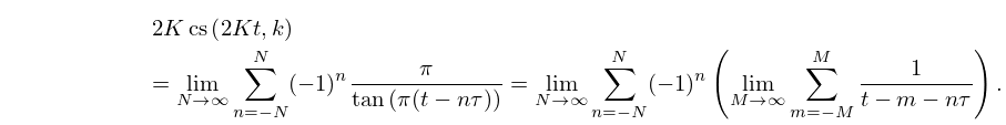
§22.12 Expansions in Other Trigonometric Series and Doubly-Infinite Partial Fractions: Eisenstein Series

►With $t\in ℂ$ and …The double sums in (22.12.2)–(22.12.4) are convergent but not absolutely convergent, hence the order of the summations is important. … ►

22.12.13 $$2K\mathrm{cs}(2Kt,k)=\underset{N\to \mathrm{\infty }}{lim}\sum _{n=-N}^N{(-1)}^n\frac{\pi }{\tan \left(\pi (t-n\tau )\right)}=\underset{N\to \mathrm{\infty }}{lim}\sum _{n=-N}^N{(-1)}^n\left(\underset{M\to \mathrm{\infty }}{lim}\sum _{m=-M}^M\frac{1}{t-m-n\tau }\right).$$

ⓘ

Symbols:

$\mathrm{cs}(z,k)$: Jacobian elliptic function, $\pi$: the ratio of the circumference of a circle to its diameter, $K\left(k\right)$: Legendre’s complete elliptic integral of the first kind, $\tan z$: tangent function, $k$: modulus and $\tau$: ratio

Referenced by:

§22.12

Permalink:

http://dlmf.nist.gov/22.12.E13

Encodings:

pMML, png, TeX

See also:

Annotations for §22.12 and Ch.22

2: 5.19 Mathematical Applications

… ►As shown in Temme (1996b, §3.4), the results given in §5.7(ii) can be used to sum infinite series of rational functions. … ►By decomposition into partial fractions (§1.2(iii)) … ►Many special functions $f(z)$ can be represented as a Mellin–Barnes integral, that is, an integral of a product of gamma functions, reciprocals of gamma functions, and a power of $z$, the integration contour being doubly-infinite and eventually parallel to the imaginary axis at both ends. …By translating the contour parallel to itself and summing the residues of the integrand, asymptotic expansions of $f(z)$ for large $|z|$, or small $|z|$, can be obtained complete with an integral representation of the error term. …

3: 31.11 Expansions in Series of Hypergeometric Functions

§31.11 Expansions in Series of Hypergeometric Functions

… ►Series of Type II (§31.11(iv)) are expansions in orthogonal polynomials, which are useful in calculations of normalization integrals for Heun functions; see Erdélyi (1944) and §31.9(i). … ►

§31.11(v) Doubly-Infinite Series

►Schmidt (1979) gives expansions of path-multiplicative solutions (§31.6) in terms of doubly-infinite series of hypergeometric functions.

4: 28.19 Expansions in Series of ${\mathrm{me}}_{\nu +2n}$ Functions

§28.19 Expansions in Series of ${\mathrm{me}}_{\nu +2n}$ Functions

►Let $q$ be a normal value (§28.12(i)) with respect to $\nu$, and $f(z)$ be a function that is analytic on a doubly-infinite open strip $S$ that contains the real axis. … ►where the coefficients are as in §28.14.

5: 28.11 Expansions in Series of Mathieu Functions

§28.11 Expansions in Series of Mathieu Functions

►Let $f(z)$ be a $2\pi$-periodic function that is analytic in an open doubly-infinite strip $S$ that contains the real axis, and $q$ be a normal value (§28.7). …See Meixner and Schäfke (1954, §2.28), and for expansions in the case of the exceptional values of $q$ see Meixner et al. (1980, p. 33). … ►

28.11.7 $$\sin (2m+2)z=\sum _{n=0}^{\mathrm{\infty }}{B}_{2m+2}^{2n+2}(q){\mathrm{se}}_{2n+2}(z,q).$$

ⓘ

Symbols:

${\mathrm{se}}_n(z,q)$: Mathieu function, $\sin z$: sine function, $m$: integer, $q=h^2$: parameter, $n$: integer, $z$: complex variable and $B_m(q)$: Fourier coefficient

Permalink:

http://dlmf.nist.gov/28.11.E7

Encodings:

pMML, png, TeX

See also:

Annotations for §28.11, §28.11 and Ch.28

6: 1.9 Calculus of a Complex Variable

… ► … ► … ►A doubly-infinite series ${\sum }_{n=-\mathrm{\infty }}^{\mathrm{\infty }}{f}_n(z)$ converges (uniformly) on $S$ iff each of the series ${\sum }_{n=0}^{\mathrm{\infty }}{f}_n(z)$ and ${\sum }_{n=1}^{\mathrm{\infty }}{f}_{-n}(z)$ converges (uniformly) on $S$. … ►Then the expansions (1.9.54), (1.9.57), and (1.9.60) hold for all sufficiently small $\left|z\right|$. …

7: 20 Theta Functions

Chapter 20 Theta Functions

…

8: 6.20 Approximations

… ►

Cody and Thacher (1968) provides minimax rational approximations for $E_1\left(x\right)$, with accuracies up to 20S.

►

Cody and Thacher (1969) provides minimax rational approximations for $\mathrm{Ei}\left(x\right)$, with accuracies up to 20S.

►

MacLeod (1996b) provides rational approximations for the sine and cosine integrals and for the auxiliary functions $\mathrm{f}$ and $\mathrm{g}$, with accuracies up to 20S.

►

§6.20(ii) Expansions in Chebyshev Series

… ►

§6.20(iii) Padé-Type and Rational Expansions

…

9: 7.24 Approximations

… ►

Cody (1969) provides minimax rational approximations for $\mathrm{erf}x$ and $\mathrm{erfc}x$. The maximum relative precision is about 20S.

… ►

Cody et al. (1970) gives minimax rational approximations to Dawson’s integral $F\left(x\right)$ (maximum relative precision 20S–22S).

►

§7.24(ii) Expansions in Chebyshev Series

… ►

Schonfelder (1978) gives coefficients of Chebyshev expansions for $x^{-1}\mathrm{erf}x$ on $0\le x\le 2$, for $x{\mathrm{e}}^{x^2}\mathrm{erfc}x$ on $[2,\mathrm{\infty })$, and for ${\mathrm{e}}^{x^2}\mathrm{erfc}x$ on $[0,\mathrm{\infty })$ (30D).

… ►

§7.24(iii) Padé-Type Expansions

…

10: 10.75 Tables

… ►

Olver (1960) tabulates $j_{n,m}$, $J_n^{\prime }\left(j_{n,m}\right)$, $j_{n,m}^{\prime }$, $J_n\left(j_{n,m}^{\prime }\right)$, $y_{n,m}$, $Y_n^{\prime }\left(y_{n,m}\right)$, $y_{n,m}^{\prime }$, $Y_n\left(y_{n,m}^{\prime }\right)$, $n=0(\frac{1}{2})20⁤\frac{1}{2}$, $m=1(1)50$, 8D. Also included are tables of the coefficients in the uniform asymptotic expansions of these zeros and associated values as $n\to \mathrm{\infty }$; see §10.21(viii), and more fully Olver (1954).

… ►

Bickley et al. (1952) tabulates $x^{-n}{I}_n\left(x\right)$ or ${\mathrm{e}}^{-x}{I}_n\left(x\right)$, $x^n{K}_n\left(x\right)$ or ${\mathrm{e}}^x{K}_n\left(x\right)$, $n=2(1)20$, $x=0$(.01 or .1) 10(.1) 20, 8S; $I_n\left(x\right)$, $K_n\left(x\right)$, $n=0(1)20$, $x=0$ or $0.1(.1)20$, 10S.

… ►

Kerimov and Skorokhodov (1984c) tabulates all zeros of $I_{-n-\frac{1}{2}}\left(z\right)$ and $I_{-n-\frac{1}{2}}^{\prime }\left(z\right)$ in the sector $0\le \mathrm{ph}z\le \frac{1}{2}\pi$ for $n=1(1)20$, 9S.

… ►

The main tables in Abramowitz and Stegun (1964, Chapter 10) give ${𝗃}_n\left(x\right)$, ${𝗒}_n\left(x\right)$ $n=0(1)8$, $x=0(.1)10$, 5–8S; ${𝗃}_n\left(x\right)$, ${𝗒}_n\left(x\right)$ $n=0(1)20(10)50$, 100, $x=1,2,5,10,50,100$, 10S; ${𝗂}_n^{(1)}\left(x\right)$, ${𝗄}_n\left(x\right)$, $n=0,1,2$, $x=0(.1)5$, 4–9D; ${𝗂}_n^{(1)}\left(x\right)$, ${𝗄}_n\left(x\right)$, $n=0(1)20(10)50$, 100, $x=1,2,5,10,50,100$, 10S. (For the notation see §10.1 and §10.47(ii).)

… ►

Olver (1960) tabulates $a_{n,m}^{\prime }$, ${𝗃}_n\left(a_{n,m}^{\prime }\right)$, $b_{n,m}^{\prime }$, ${𝗒}_n\left(b_{n,m}^{\prime }\right)$, $n=1(1)20$, $m=1(1)50$, 8D. Also included are tables of the coefficients in the uniform asymptotic expansions of these zeros and associated values as $n\to \mathrm{\infty }$.

…