eta%20function
(0.002 seconds)
8 matching pages
1: 33.24 Tables
§33.24 Tables
►Abramowitz and Stegun (1964, Chapter 14) tabulates , , , and for and , 5S; for , 6S.
2: 33.3 Graphics
§33.3 Graphics
►§33.3(i) Line Graphs of the Coulomb Radial Functions and
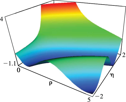
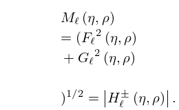
… ►§33.3(ii) Surfaces of the Coulomb Radial Functions and
… ►
3: 10.75 Tables
The main tables in Abramowitz and Stegun (1964, Chapter 9) give to 15D, , , , to 10D, to 8D, ; , , , 8D; , , , , 5D or 5S; , , , , 10S; modulus and phase functions , , , , 8D.
Achenbach (1986) tabulates , , , , , 20D or 18–20S.
British Association for the Advancement of Science (1937) tabulates , , , 7–8D; , , , 7–10D; , , , , , 8D. Also included are auxiliary functions to facilitate interpolation of the tables of , for small values of .
Bickley et al. (1952) tabulates or , or , , (.01 or .1) 10(.1) 20, 8S; , , , or , 10S.
Zhang and Jin (1996, pp. 296–305) tabulates , , , , , , , , , 50, 100, , 5, 10, 25, 50, 100, 8S; , , , (Riccati–Bessel functions and their derivatives), , 50, 100, , 5, 10, 25, 50, 100, 8S; real and imaginary parts of , , , , , , , , , 20(10)50, 100, , , 8S. (For the notation replace by , , , , respectively.)
