eta function

AdvancedHelp

(0.002 seconds)

1—10 of 73 matching pages

1: 23.16 Graphics
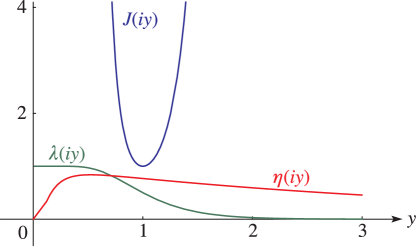
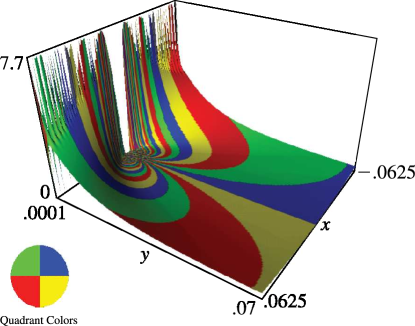
… ►See Figures 23.16.1–23.16.3 for the modular functions λ , J , and η . … ►
►See accompanying text►
Figure 23.16.1: Modular functions λ ⁡ ( i ⁢ y ) , J ⁡ ( i ⁢ y ) , η ⁡ ( i ⁢ y ) for 0 ≤ y ≤ 3 . … Magnify
… ►
►
See accompanying text
►
Figure 23.16.3: Dedekind’s eta function η ⁡ ( x + i ⁢ y ) for − 0.0625 ≤ x ≤ 0.0625 , 0.0001 ≤ y ≤ 0.07 . Magnify 3D Help
2: 23.15 Definitions
… ►
§23.15(ii) Functions λ ⁡ ( τ ) , J ⁡ ( τ ) , η ⁡ ( τ )
… ►
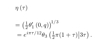
Dedekind’s Eta Function (or Dedekind Modular Function)
► …
3: 23.19 Interrelations
… ►
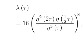
23.19.1 λ ⁡ ( τ ) = 16 ⁢ ( η 2 ⁡ ( 2 ⁢ τ ) ⁢ η ⁡ ( 1 2 ⁢ τ ) η 3 ⁡ ( τ ) ) 8 ,
… ►
4: 23.1 Special Notation
… ►The main functions treated in this chapter are the Weierstrass ℘ -function ℘ ⁡ ( z ) = ℘ ⁡ ( z | 𝕃 ) = ℘ ⁡ ( z ; g 2 ⁡ , g 3 ⁡ ) ; the Weierstrass zeta function ζ ⁡ ( z ) = ζ ⁡ ( z | 𝕃 ) = ζ ⁡ ( z ; g 2 ⁡ , g 3 ⁡ ) ; the Weierstrass sigma function σ ⁡ ( z ) = σ ⁡ ( z | 𝕃 ) = σ ⁡ ( z ; g 2 ⁡ , g 3 ⁡ ) ; the elliptic modular function λ ⁡ ( τ ) ; Klein’s complete invariant J ⁡ ( τ ) ; Dedekind’s eta function η ⁡ ( τ ) . …
5: 8.12 Uniform Asymptotic Expansions for Large Parameter
… ►
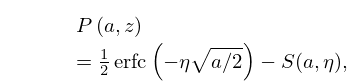
8.12.3 P ⁡ ( a , z ) = 1 2 ⁢ erfc ⁡ ( − η ⁢ a / 2 ) − S ⁡ ( a , η ) ,
►
8.12.4 Q ⁡ ( a , z ) = 1 2 ⁢ erfc ⁡ ( η ⁢ a / 2 ) + S ⁡ ( a , η ) ,
… ►Then as a → ∞ in the sector | ph ⁡ a | ≤ π − δ ( < π ) , ►
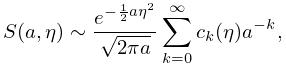
8.12.7 S ⁡ ( a , η ) ∼ e − 1 2 ⁢ a ⁢ η 2 2 ⁢ π ⁢ a ⁢ ∑ k = 0 ∞ c k ⁡ ( η ) ⁢ a − k ,
►
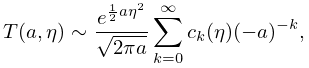
8.12.8 T ⁡ ( a , η ) ∼ e 1 2 ⁢ a ⁢ η 2 2 ⁢ π ⁢ a ⁢ ∑ k = 0 ∞ c k ⁡ ( η ) ⁢ ( − a ) − k ,
…
6: 33.11 Asymptotic Expansions for Large ρ
§33.11 Asymptotic Expansions for Large ρ
… ►
33.11.1 H ℓ ± ⁡ ( η , ρ ) ∼ e ± i ⁢ θ ℓ ⁡ ( η , ρ ) ⁢ ∑ k = 0 ∞ ( a ) k ⁢ ( b ) k k ! ⁢ ( ± 2 ⁢ i ⁢ ρ ) k ,
… ►
33.11.4 H ℓ ± ⁡ ( η , ρ ) = e ± i ⁢ θ ℓ ⁢ ( f ⁡ ( η , ρ ) ± i ⁢ g ⁡ ( η , ρ ) ) ,
… ►
33.11.7 g ⁡ ( η , ρ ) ⁢ f ^ ⁡ ( η , ρ ) − f ⁡ ( η , ρ ) ⁢ g ^ ⁡ ( η , ρ ) = 1 .
…
7: 33.2 Definitions and Basic Properties
… ►
§33.2(ii) Regular Solution F ℓ ⁡ ( η , ρ )
… ► F ℓ ⁡ ( η , ρ ) is a real and analytic function of ρ on the open interval 0 < ρ < ∞ , and also an analytic function of η when − ∞ < η < ∞ . … ►
§33.2(iii) Irregular Solutions G ℓ ⁡ ( η , ρ ) , H ℓ ± ⁡ ( η , ρ )
… ►Also, e ∓ i ⁢ σ ℓ ⁡ ( η ) ⁢ H ℓ ± ⁡ ( η , ρ ) are analytic functions of η when − ∞ < η < ∞ . ►
§33.2(iv) Wronskians and Cross-Product
…
8: 23.17 Elementary Properties
… ►
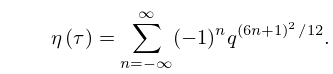
23.17.6 η ⁡ ( τ ) = ∑ n = − ∞ ∞ ( − 1 ) n ⁢ q ( 6 ⁢ n + 1 ) 2 / 12 .
… ►
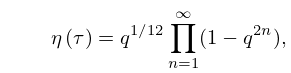
23.17.8 η ⁡ ( τ ) = q 1 / 12 ⁢ ∏ n = 1 ∞ ( 1 − q 2 ⁢ n ) ,
…
9: 27.14 Unrestricted Partitions
… ►Dedekind sums occur in the transformation theory of the Dedekind modular function η ⁡ ( τ ) , defined by ►
27.14.12 η ⁡ ( τ ) = e π ⁢ i ⁢ τ / 12 ⁢ ∏ n = 1 ∞ ( 1 − e 2 ⁢ π ⁢ i ⁢ n ⁢ τ ) , ℑ ⁡ τ > 0 .
… ► η ⁡ ( τ ) satisfies the following functional equation: if a , b , c , d are integers with a ⁢ d − b ⁢ c = 1 and c > 0 , then … ►For further properties of the function η ⁡ ( τ ) see §§23.15–23.19. … ►
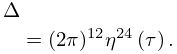
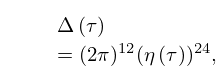
27.14.16 Δ ⁡ ( τ ) = ( 2 ⁢ π ) 12 ⁢ ( η ⁡ ( τ ) ) 24 , ℑ ⁡ τ > 0 ,
…
10: 23.18 Modular Transformations
… ►
Dedekind’s Eta Function
►
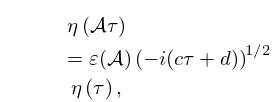
23.18.5 η ⁡ ( 𝒜 τ ) = ε ⁡ ( 𝒜 ) ⁢ ( − i ⁢ ( c ⁢ τ + d ) ) 1 / 2 ⁢ η ⁡ ( τ ) ,
…