equianharmonic
♦
4 matching pages ♦
(0.002 seconds)
4 matching pages
1: 23.4 Graphics
…
►
► ►
►
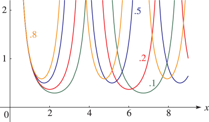
Figure 23.4.2:
for , = 0.
…(Equianharmonic case.)
Magnify
…
►
► ►
►
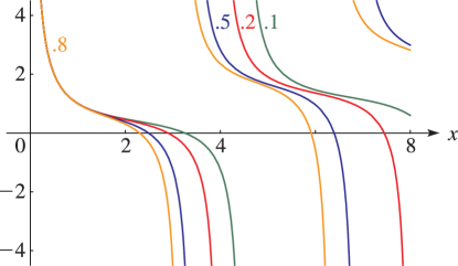
Figure 23.4.4:
for , = 0.
…(Equianharmonic case.)
Magnify
…
►
► ►
►
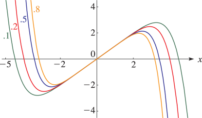
Figure 23.4.6:
for , = 0.
…(Equianharmonic case.)
Magnify
…
§23.4(i) Real Variables
►Line graphs of the Weierstrass functions , , and , illustrating the lemniscatic and equianharmonic cases. … ►►
►
►
2: 23.5 Special Lattices
3: 22.5 Special Values
…
►For values of when (lemniscatic case) see §23.5(iii), and for (equianharmonic case) see §23.5(v).
4: 23.22 Methods of Computation
…
►
(c)
…
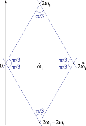
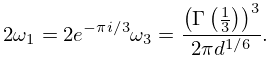
If , then
23.22.3
There are 6 possible pairs (, ), corresponding to the 6 rotations of a lattice of equilateral triangles. The equianharmonic case occurs when and .
