equation of Ince

SearchAdvancedHelp

(0.002 seconds)

11—17 of 17 matching pages

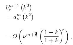
11: 29.7 Asymptotic Expansions

… ►

29.7.1 $$a_{\nu }^m\left(k^2\right)\sim p\kappa -{\tau }_0-{\tau }_1{\kappa }^{-1}-{\tau }_2{\kappa }^{-2}-\mathrm{\cdots },$$

ⓘ

Symbols:

$a_{\nu }^n\left(k^2\right)$: eigenvalues of Lamé’s equation, $\sim$: Poincaré asymptotic expansion, $m$: nonnegative integer, $p$: nonnegative integer, $k$: real parameter, $\nu$: real parameter, $\kappa$ and ${\tau }_j$: coefficients

Permalink:

http://dlmf.nist.gov/29.7.E1

Encodings:

pMML, png, TeX

See also:

Annotations for §29.7(i), §29.7 and Ch.29

… ►

29.7.5 $$b_{\nu }^{m+1}\left(k^2\right)-a_{\nu }^m\left(k^2\right)=O\left({\nu }^{m+\frac{3}{2}}{\left(\frac{1-k}{1+k}\right)}^{\nu }\right),$$ $\nu \to \mathrm{\infty }$.

ⓘ

Symbols:

$O\left(x\right)$: order not exceeding, $a_{\nu }^n\left(k^2\right)$: eigenvalues of Lamé’s equation, $b_{\nu }^n\left(k^2\right)$: eigenvalues of Lamé’s equation, $m$: nonnegative integer, $k$: real parameter and $\nu$: real parameter

Referenced by:

§29.7(i)

Permalink:

http://dlmf.nist.gov/29.7.E5

Encodings:

pMML, png, TeX

See also:

Annotations for §29.7(i), §29.7 and Ch.29

… ►Weinstein and Keller (1985) give asymptotics for solutions of Hill’s equation (§28.29(i)) that are applicable to the Lamé equation.

12: 29.21 Tables

… ►

Ince (1940a) tabulates the eigenvalues $a_{\nu }^m\left(k^2\right)$, $b_{\nu }^{m+1}\left(k^2\right)$ (with $a_{\nu }^{2m+1}$ and $b_{\nu }^{2m+1}$ interchanged) for $k^2=0.1,0.5,0.9$, $\nu =-\frac{1}{2},0(1)25$, and $m=0,1,2,3$. Precision is 4D.

►

Arscott and Khabaza (1962) tabulates the coefficients of the polynomials $P$ in Table 29.12.1 (normalized so that the numerically largest coefficient is unity, i.e. monic polynomials), and the corresponding eigenvalues $h$ for $k^2=0.1(.1)0.9$, $n=1(1)30$. Equations from §29.6 can be used to transform to the normalization adopted in this chapter. Precision is 6S.

13: 29.15 Fourier Series and Chebyshev Series

… ►Equations (29.6.4), with $p=1,2,\mathrm{\dots },n$, (29.6.3), and $A_{2n+2}=0$ can be cast as an algebraic eigenvalue problem in the following way. … ►

29.15.7 $$a_{\nu }^{2m}\left(k^2\right)=\frac{1}{2}(H_m+\nu (\nu +1)k^2),$$

ⓘ

Symbols:

$a_{\nu }^n\left(k^2\right)$: eigenvalues of Lamé’s equation, $m$: nonnegative integer, $k$: real parameter, $\nu$: real parameter and $H_p$: eigenvalues

Permalink:

http://dlmf.nist.gov/29.15.E7

Encodings:

pMML, png, TeX

See also:

Annotations for §29.15(i), §29.15(i), §29.15 and Ch.29

… ►

29.15.12 $$a_{\nu }^{2m+1}\left(k^2\right)=\frac{1}{2}(H_m+\nu (\nu +1)k^2),$$

ⓘ

Symbols:

$a_{\nu }^n\left(k^2\right)$: eigenvalues of Lamé’s equation, $m$: nonnegative integer, $k$: real parameter, $\nu$: real parameter and $H_p$: eigenvalues

Permalink:

http://dlmf.nist.gov/29.15.E12

Encodings:

pMML, png, TeX

See also:

Annotations for §29.15(i), §29.15(i), §29.15 and Ch.29

… ►

29.15.17 $$b_{\nu }^{2m+1}\left(k^2\right)=\frac{1}{2}(H_m+\nu (\nu +1)k^2),$$

ⓘ

Symbols:

$b_{\nu }^n\left(k^2\right)$: eigenvalues of Lamé’s equation, $m$: nonnegative integer, $k$: real parameter, $\nu$: real parameter and $H_p$: eigenvalues

Permalink:

http://dlmf.nist.gov/29.15.E17

Encodings:

pMML, png, TeX

See also:

Annotations for §29.15(i), §29.15(i), §29.15 and Ch.29

… ►

29.15.22 $$a_{\nu }^{2m}\left(k^2\right)=\frac{1}{2}(H_m+\nu (\nu +1)k^2),$$

ⓘ

Symbols:

$a_{\nu }^n\left(k^2\right)$: eigenvalues of Lamé’s equation, $m$: nonnegative integer, $k$: real parameter, $\nu$: real parameter and $H_p$: eigenvalues

Permalink:

http://dlmf.nist.gov/29.15.E22

Encodings:

pMML, png, TeX

See also:

Annotations for §29.15(i), §29.15(i), §29.15 and Ch.29

…

14: 29.17 Other Solutions

… ►

§29.17(i) Second Solution

… ►See Erdélyi (1941c), Ince (1940b), and Lambe (1952). …

15: 28.35 Tables

§28.35 Tables

… ►

Ince (1932) includes eigenvalues $a_n$, $b_n$, and Fourier coefficients for $n=0$ or $1(1)6$, $q=0(1)10(2)20(4)40$; 7D. Also ${\mathrm{ce}}_n(x,q)$, ${\mathrm{se}}_n(x,q)$ for $q=0(1)10$, $x=1(1)90$, corresponding to the eigenvalues in the tables; 5D. Notation: $a_n={\mathrm{𝑏𝑒}}_n-2q$, $b_n={\mathrm{𝑏𝑜}}_n-2q$.

… ►

Blanch and Clemm (1969) includes eigenvalues $a_n\left(q\right)$, $b_n\left(q\right)$ for $q=\rho {\mathrm{e}}^{\mathrm{i}\varphi }$, $\rho =0(.5)25$, $\varphi =5^{\circ }(5^{\circ }){90}^{\circ }$, $n=0(1)15$; 4D. Also $a_n\left(q\right)$ and $b_n\left(q\right)$ for $q=\mathrm{i}\rho$, $\rho =0(.5)100$, $n=0(2)14$ and $n=2(2)16$, respectively; 8D. Double points for $n=0(1)15$; 8D. Graphs are included.

… ►

Ince (1932) includes the first zero for ${\mathrm{ce}}_n$, ${\mathrm{se}}_n$ for $n=2(1)5$ or $6$, $q=0(1)10(2)40$; 4D. This reference also gives zeros of the first derivatives, together with expansions for small $q$.

…

16: 29.6 Fourier Series

… ►

29.6.2 $$H=2a_{\nu }^{2m}\left(k^2\right)-\nu (\nu +1)k^2,$$

ⓘ

Defines:

$H$ (locally)

Symbols:

$a_{\nu }^n\left(k^2\right)$: eigenvalues of Lamé’s equation, $m$: nonnegative integer, $k$: real parameter and $\nu$: real parameter

Referenced by:

§29.6(i)

Permalink:

http://dlmf.nist.gov/29.6.E2

Encodings:

pMML, png, TeX

See also:

Annotations for §29.6(i), §29.6 and Ch.29

… ►

29.6.17 $$H=2a_{\nu }^{2m+1}\left(k^2\right)-\nu (\nu +1)k^2,$$

ⓘ

Defines:

$H$ (locally)

Symbols:

$a_{\nu }^n\left(k^2\right)$: eigenvalues of Lamé’s equation, $m$: nonnegative integer, $k$: real parameter and $\nu$: real parameter

Permalink:

http://dlmf.nist.gov/29.6.E17

Encodings:

pMML, png, TeX

See also:

Annotations for §29.6(ii), §29.6 and Ch.29

… ►

29.6.32 $$H=2b_{\nu }^{2m+1}\left(k^2\right)-\nu (\nu +1)k^2,$$

ⓘ

Defines:

$H$ (locally)

Symbols:

$b_{\nu }^n\left(k^2\right)$: eigenvalues of Lamé’s equation, $m$: nonnegative integer, $k$: real parameter and $\nu$: real parameter

Permalink:

http://dlmf.nist.gov/29.6.E32

Encodings:

pMML, png, TeX

See also:

Annotations for §29.6(iii), §29.6 and Ch.29

… ►

29.6.47 $$H=2b_{\nu }^{2m+2}\left(k^2\right)-\nu (\nu +1)k^2,$$

ⓘ

Defines:

$H$ (locally)

Symbols:

$b_{\nu }^n\left(k^2\right)$: eigenvalues of Lamé’s equation, $m$: nonnegative integer, $k$: real parameter and $\nu$: real parameter

Permalink:

http://dlmf.nist.gov/29.6.E47

Encodings:

pMML, png, TeX

See also:

Annotations for §29.6(iv), §29.6 and Ch.29

…

17: 29.1 Special Notation

… ►Other notations that have been used are as follows: Ince (1940a) interchanges $a_{\nu }^{2m+1}\left(k^2\right)$ with $b_{\nu }^{2m+1}\left(k^2\right)$. …The relation to the Lamé functions ${\mathrm{Ec}}_{\nu }^m$, ${\mathrm{Es}}_{\nu }^m$ of Ince (1940b) is given by … ►

$${(s_{\nu }^m(k^2))}^2=\frac{4}{\pi }{\int }_0^K{\left({\mathrm{𝐸𝑠}}_{\nu }^m(x,k^2)\right)}^{2}dx.$$