eigenvalues of accessory parameter

SearchAdvancedHelp

(0.003 seconds)

1—10 of 415 matching pages

1: 31.13 Asymptotic Approximations

§31.13 Asymptotic Approximations

►For asymptotic approximations for the accessory parameter eigenvalues $q_m$, see Fedoryuk (1991) and Slavyanov (1996). …

2: 31.4 Solutions Analytic at Two Singularities: Heun Functions

… ►For an infinite set of discrete values $q_m$, $m=0,1,2,\mathrm{\dots }$, of the accessory parameter $q$, the function $H\mathrm{\ell }(a,q;\alpha ,\beta ,\gamma ,\delta ;z)$ is analytic at $z=1$, and hence also throughout the disk . … ►

31.4.1 $$(0,1){\mathrm{𝐻𝑓}}_m(a,q_m;\alpha ,\beta ,\gamma ,\delta ;z),$$ $m=0,1,2,\mathrm{\dots }$.

ⓘ

Symbols:

$(s_1,s_2){\mathrm{𝐻𝑓}}_m(a,q_m;\alpha ,\beta ,\gamma ,\delta ;z)$: Heun functions, $z$: complex variable, $\gamma$: real or complex parameter, $\delta$: real or complex parameter, $m$: nonnegative integer, $a$: complex parameter, $q$: real or complex parameter, $\alpha$: real or complex parameter and $\beta$: real or complex parameter

Referenced by:

§31.6

Permalink:

http://dlmf.nist.gov/31.4.E1

Encodings:

pMML, png, TeX

See also:

Annotations for §31.4 and Ch.31

►The eigenvalues $q_m$ satisfy the continued-fraction equation ►

31.4.2 $$q=\frac{a\gamma P_1}{Q_1+q-}\frac{R_1{P}_2}{Q_2+q-}\frac{R_2{P}_3}{Q_3+q-}\mathrm{\cdots },$$

ⓘ

Symbols:

$\gamma$: real or complex parameter, $a$: complex parameter, $q$: real or complex parameter, $P_j$: coefficient, $Q_j$: coefficient and $R_j$: coefficient

Referenced by:

§31.18

Permalink:

http://dlmf.nist.gov/31.4.E2

Encodings:

pMML, png, TeX

See also:

Annotations for §31.4 and Ch.31

… ►

31.4.3 $$(s_1,s_2){\mathrm{𝐻𝑓}}_m(a,q_m;\alpha ,\beta ,\gamma ,\delta ;z),$$ $m=0,1,2,\mathrm{\dots }$,

ⓘ

Symbols:

$(s_1,s_2){\mathrm{𝐻𝑓}}_m(a,q_m;\alpha ,\beta ,\gamma ,\delta ;z)$: Heun functions, $z$: complex variable, $\gamma$: real or complex parameter, $\delta$: real or complex parameter, $m$: nonnegative integer, $a$: complex parameter, $q$: real or complex parameter, $\alpha$: real or complex parameter and $\beta$: real or complex parameter

Referenced by:

§31.4, §31.6

Permalink:

http://dlmf.nist.gov/31.4.E3

Encodings:

pMML, png, TeX

See also:

Annotations for §31.4 and Ch.31

…

3: 28.7 Analytic Continuation of Eigenvalues

§28.7 Analytic Continuation of Eigenvalues

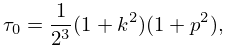
►As functions of $q$, $a_n\left(q\right)$ and $b_n\left(q\right)$ can be continued analytically in the complex $q$-plane. The only singularities are algebraic branch points, with $a_n\left(q\right)$ and $b_n\left(q\right)$ finite at these points. …The normal values are simple roots of the corresponding equations (28.2.21) and (28.2.22). … ► …

4: 29.4 Graphics

… ►

§29.4(i) Eigenvalues of Lamé’s Equation: Line Graphs

►

►►

Figure 29.4.1: $a_{\nu }^m\left(0.5\right)$, $b_{\nu }^{m+1}\left(0.5\right)$ as functions of $\nu$ for $m=0,1,2,3$. Magnify

►

►►

Figure 29.4.2: $a_{\nu }^3\left(0.5\right)-b_{\nu }^3\left(0.5\right)$ as a function of $\nu$. Magnify

… ►

§29.4(ii) Eigenvalues of Lamé’s Equation: Surfaces

… ►

►

►

Figure 29.4.12: $b_{\nu }^2\left(k^2\right)$ as a function of $\nu$ and $k^2$. Magnify 3D Help

…

5: 28.13 Graphics

… ►

§28.13(i) Eigenvalues ${\lambda }_{\nu }\left(q\right)$ for General $\nu$

►

►►

Figure 28.13.1: ${\lambda }_{\nu }\left(q\right)$ as a function of $q$ for $\nu =0.5(1)3.5$ and $a_n\left(q\right),b_n\left(q\right)$ for $n=0,1,2,3,4$ ($a$’s), $n=1,2,3,4$ ($b$’s). … Magnify

►

►

►

Figure 28.13.2: ${\lambda }_{\nu }\left(q\right)$ for , $0\le q\le 10$. Magnify 3D Help

…

6: 28.6 Expansions for Small $q$

… ►

§28.6(i) Eigenvalues

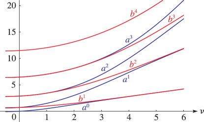
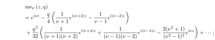
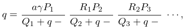
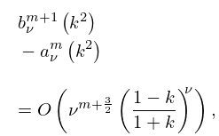
►Leading terms of the power series for $a_m\left(q\right)$ and $b_m\left(q\right)$ for $m\le 6$ are: … ►The coefficients of the power series of $a_{2n}\left(q\right)$, $b_{2n}\left(q\right)$ and also $a_{2n+1}\left(q\right)$, $b_{2n+1}\left(q\right)$ are the same until the terms in $q^{2n-2}$ and $q^{2n}$, respectively. … ►Higher coefficients in the foregoing series can be found by equating coefficients in the following continued-fraction equations: … ►Here $j=1$ for $a_{2n}\left(q\right)$, $j=2$ for $b_{2n+2}\left(q\right)$, and $j=3$ for $a_{2n+1}\left(q\right)$ and $b_{2n+1}\left(q\right)$. …

7: 28.34 Methods of Computation

… ►

§28.34(ii) Eigenvalues

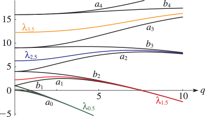
►Methods for computing the eigenvalues $a_n\left(q\right)$, $b_n\left(q\right)$, and ${\lambda }_{\nu }\left(q\right)$, defined in §§28.2(v) and 28.12(i), include: … ►

Solution of the matrix eigenvalue problem for each of the five infinite matrices that correspond to the linear algebraic equations (28.4.5)–(28.4.8) and (28.14.4). See Zhang and Jin (1996, pp. 479–482) and §3.2(iv).

… ►

Asymptotic approximations by zeros of orthogonal polynomials of increasing degree. See Volkmer (2008). This method also applies to eigenvalues of the Whittaker–Hill equation (§28.31(i)) and eigenvalues of Lamé functions (§29.3(i)).

… ►Also, once the eigenvalues $a_n\left(q\right)$, $b_n\left(q\right)$, and ${\lambda }_{\nu }\left(q\right)$ have been computed the following methods are applicable: …

8: 29.3 Definitions and Basic Properties

… ►

§29.3(i) Eigenvalues

… ►

§29.3(ii) Distribution

►The eigenvalues interlace according to …The eigenvalues coalesce according to … ►

§29.3(vii) Power Series

…

9: 28.15 Expansions for Small $q$

… ►

§28.15(i) Eigenvalues ${\lambda }_{\nu }\left(q\right)$

►

28.15.1 $${\lambda }_{\nu }\left(q\right)={\nu }^2+\frac{1}{2({\nu }^2-1)}{q}^2+\frac{5{\nu }^2+7}{32{({\nu }^2-1)}^3({\nu }^2-4)}{q}^4+\frac{9{\nu }^4+58{\nu }^2+29}{64{({\nu }^2-1)}^5({\nu }^2-4)({\nu }^2-9)}{q}^6+\mathrm{\cdots }.$$

ⓘ

Symbols:

${\lambda }_{\nu +2n}\left(q\right)$: eigenvalues of Mathieu equation, $q=h^2$: parameter and $\nu$: complex parameter

A&S Ref:

20.3.15 (in slightly different form)

Permalink:

http://dlmf.nist.gov/28.15.E1

Encodings:

pMML, png, TeX

See also:

Annotations for §28.15(i), §28.15 and Ch.28

►Higher coefficients can be found by equating powers of $q$ in the following continued-fraction equation, with $a={\lambda }_{\nu }\left(q\right)$: ►

28.15.2 $$a-{\nu }^2-\frac{q^2}{a-{(\nu +2)}^2-}\frac{q^2}{a-{(\nu +4)}^2-}\mathrm{\cdots }=\frac{q^2}{a-{(\nu -2)}^2-}\frac{q^2}{a-{(\nu -4)}^2-}\mathrm{\cdots }.$$

ⓘ

Symbols:

$q=h^2$: parameter, $\nu$: complex parameter and $a$: parameter

Referenced by:

item (e)

Permalink:

http://dlmf.nist.gov/28.15.E2

Encodings:

pMML, png, TeX

See also:

Annotations for §28.15(i), §28.15 and Ch.28

… ►

28.15.3 $${\mathrm{me}}_{\nu }(z,q)={\mathrm{e}}^{\mathrm{i}\nu z}-\frac{q}{4}\left(\frac{1}{\nu +1}{\mathrm{e}}^{\mathrm{i}(\nu +2)z}-\frac{1}{\nu -1}{\mathrm{e}}^{\mathrm{i}(\nu -2)z}\right)+\frac{q^2}{32}\left(\frac{1}{(\nu +1)(\nu +2)}{\mathrm{e}}^{\mathrm{i}(\nu +4)z}+\frac{1}{(\nu -1)(\nu -2)}{\mathrm{e}}^{\mathrm{i}(\nu -4)z}-\frac{2({\nu }^2+1)}{{({\nu }^2-1)}^2}{\mathrm{e}}^{\mathrm{i}\nu z}\right)+\mathrm{\cdots };$$

ⓘ

Symbols:

${\mathrm{me}}_n(z,q)$: Mathieu function, $\mathrm{e}$: base of natural logarithm, $\mathrm{i}$: imaginary unit, $q=h^2$: parameter, $z$: complex variable and $\nu$: complex parameter

A&S Ref:

20.3.17 (only two terms and without normalization)

Permalink:

http://dlmf.nist.gov/28.15.E3

Encodings:

pMML, png, TeX

See also:

Annotations for §28.15(ii), §28.15 and Ch.28

…

10: 29.7 Asymptotic Expansions

… ►

§29.7(i) Eigenvalues

… ►

29.7.1 $$a_{\nu }^m\left(k^2\right)\sim p\kappa -{\tau }_0-{\tau }_1{\kappa }^{-1}-{\tau }_2{\kappa }^{-2}-\mathrm{\cdots },$$

ⓘ

Symbols:

$a_{\nu }^n\left(k^2\right)$: eigenvalues of Lamé’s equation, $\sim$: Poincaré asymptotic expansion, $m$: nonnegative integer, $p$: nonnegative integer, $k$: real parameter, $\nu$: real parameter, $\kappa$ and ${\tau }_j$: coefficients

Permalink:

http://dlmf.nist.gov/29.7.E1

Encodings:

pMML, png, TeX

See also:

Annotations for §29.7(i), §29.7 and Ch.29

… ►

29.7.3 $${\tau }_0=\frac{1}{2^3}(1+k^2)(1+p^2),$$

ⓘ

Symbols:

$p$: nonnegative integer, $k$: real parameter and ${\tau }_j$: coefficients

Permalink:

http://dlmf.nist.gov/29.7.E3

Encodings:

pMML, png, TeX

See also:

Annotations for §29.7(i), §29.7 and Ch.29

… ►The same Poincaré expansion holds for $b_{\nu }^{m+1}\left(k^2\right)$, since ►

29.7.5 $$b_{\nu }^{m+1}\left(k^2\right)-a_{\nu }^m\left(k^2\right)=O\left({\nu }^{m+\frac{3}{2}}{\left(\frac{1-k}{1+k}\right)}^{\nu }\right),$$ $\nu \to \mathrm{\infty }$.

ⓘ

Symbols:

$O\left(x\right)$: order not exceeding, $a_{\nu }^n\left(k^2\right)$: eigenvalues of Lamé’s equation, $b_{\nu }^n\left(k^2\right)$: eigenvalues of Lamé’s equation, $m$: nonnegative integer, $k$: real parameter and $\nu$: real parameter

Referenced by:

§29.7(i)

Permalink:

http://dlmf.nist.gov/29.7.E5

Encodings:

pMML, png, TeX

See also:

Annotations for §29.7(i), §29.7 and Ch.29

…