eigenvalue%2Feigenvector%20characterization

SearchAdvancedHelp

The term"feigenvector" was not found.Possible alternative term: "eigenvector".

(0.006 seconds)

1—10 of 823 matching pages

1: 28.7 Analytic Continuation of Eigenvalues

§28.7 Analytic Continuation of Eigenvalues

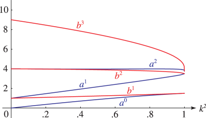
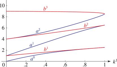
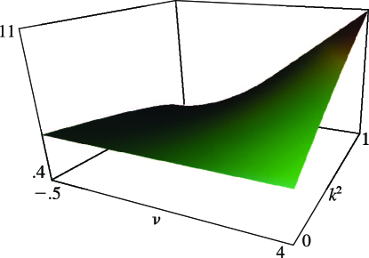
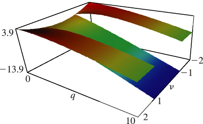
… ►To 4D the first branch points between $a_0\left(q\right)$ and $a_2\left(q\right)$ are at $q_0=\pm \mathrm{i}1.4688$ with $a_0\left(q_0\right)=a_2\left(q_0\right)=2.0886$, and between $b_2\left(q\right)$ and $b_4\left(q\right)$ they are at $q_1=\pm \mathrm{i}6.9289$ with $b_2\left(q_1\right)=b_4\left(q_1\right)=11.1904$. … ►For a visualization of the first branch point of $a_0\left(\mathrm{i}\widehat{q}\right)$ and $a_2\left(\mathrm{i}\widehat{q}\right)$ see Figure 28.7.1. 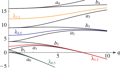… ►All the $a_{2n}\left(q\right)$, $n=0,1,2,\mathrm{\dots }$, can be regarded as belonging to a complete analytic function (in the large). …Analogous statements hold for $a_{2n+1}\left(q\right)$, $b_{2n+1}\left(q\right)$, and $b_{2n+2}\left(q\right)$, also for $n=0,1,2,\mathrm{\dots }$. …

2: 29.21 Tables

… ►

Ince (1940a) tabulates the eigenvalues $a_{\nu }^m\left(k^2\right)$, $b_{\nu }^{m+1}\left(k^2\right)$ (with $a_{\nu }^{2m+1}$ and $b_{\nu }^{2m+1}$ interchanged) for $k^2=0.1,0.5,0.9$, $\nu =-\frac{1}{2},0(1)25$, and $m=0,1,2,3$. Precision is 4D.

►

Arscott and Khabaza (1962) tabulates the coefficients of the polynomials $P$ in Table 29.12.1 (normalized so that the numerically largest coefficient is unity, i.e. monic polynomials), and the corresponding eigenvalues $h$ for $k^2=0.1(.1)0.9$, $n=1(1)30$. Equations from §29.6 can be used to transform to the normalization adopted in this chapter. Precision is 6S.

3: 29.20 Methods of Computation

… ►

§29.20(i) Lamé Functions

►The eigenvalues $a_{\nu }^m\left(k^2\right)$, $b_{\nu }^m\left(k^2\right)$, and the Lamé functions ${\mathrm{𝐸𝑐}}_{\nu }^m(z,k^2)$, ${\mathrm{𝐸𝑠}}_{\nu }^m(z,k^2)$, can be calculated by direct numerical methods applied to the differential equation (29.2.1); see §3.7. … ►A third method is to approximate eigenvalues and Fourier coefficients of Lamé functions by eigenvalues and eigenvectors of finite matrices using the methods of §§3.2(vi) and 3.8(iv). … ►

§29.20(ii) Lamé Polynomials

►The eigenvalues corresponding to Lamé polynomials are computed from eigenvalues of the finite tridiagonal matrices $𝐌$ given in §29.15(i), using methods described in §3.2(vi) and Ritter (1998). …

4: 29.9 Stability

… ►If $\nu$ is not an integer, then (29.2.1) is unstable iff $h\le a_{\nu }^0\left(k^2\right)$ or $h$ lies in one of the closed intervals with endpoints $a_{\nu }^m\left(k^2\right)$ and $b_{\nu }^m\left(k^2\right)$, $m=1,2,\mathrm{\dots }$. If $\nu$ is a nonnegative integer, then (29.2.1) is unstable iff $h\le a_{\nu }^0\left(k^2\right)$ or $h\in [b_{\nu }^m\left(k^2\right),a_{\nu }^m\left(k^2\right)]$ for some $m=1,2,\mathrm{\dots },\nu$.

5: 29.4 Graphics

… ►

§29.4(i) Eigenvalues of Lamé’s Equation: Line Graphs

… ►

►►

Figure 29.4.3: $a_{1.5}^m\left(k^2\right)$, $b_{1.5}^{m+1}\left(k^2\right)$ as functions of $k^2$ for $m=0,1,2$. Magnify

… ►

►►

Figure 29.4.8: $a_{2.5}^m\left(k^2\right)$, $b_{2.5}^{m+1}\left(k^2\right)$ as functions of $k^2$ for $m=0,1,2$. Magnify

►

§29.4(ii) Eigenvalues of Lamé’s Equation: Surfaces

… ►

►

►

Figure 29.4.12: $b_{\nu }^2\left(k^2\right)$ as a function of $\nu$ and $k^2$. Magnify 3D Help

…

6: 28.6 Expansions for Small $q$

… ►

§28.6(i) Eigenvalues

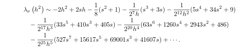
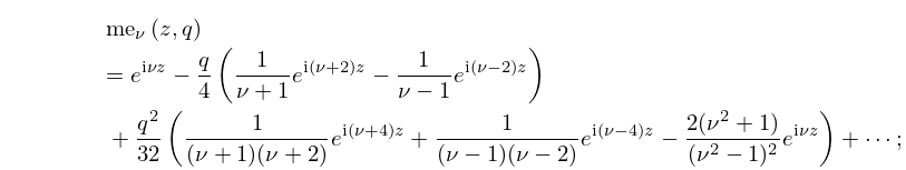
►Leading terms of the power series for $a_m\left(q\right)$ and $b_m\left(q\right)$ for $m\le 6$ are: … ►The coefficients of the power series of $a_{2n}\left(q\right)$, $b_{2n}\left(q\right)$ and also $a_{2n+1}\left(q\right)$, $b_{2n+1}\left(q\right)$ are the same until the terms in $q^{2n-2}$ and $q^{2n}$, respectively. … ►Higher coefficients in the foregoing series can be found by equating coefficients in the following continued-fraction equations: … ►Here $j=1$ for $a_{2n}\left(q\right)$, $j=2$ for $b_{2n+2}\left(q\right)$, and $j=3$ for $a_{2n+1}\left(q\right)$ and $b_{2n+1}\left(q\right)$. …

7: 28.16 Asymptotic Expansions for Large $q$

§28.16 Asymptotic Expansions for Large $q$

►Let $s=2m+1$, $m=0,1,2,\mathrm{\dots }$, and $\nu$ be fixed with . … ►

28.16.1 $${\lambda }_{\nu }\left(h^2\right)\sim -2h^2+2sh-\frac{1}{8}(s^2+1)-\frac{1}{2^{7}h}(s^3+3s)-\frac{1}{2^{12}{h}^2}(5s^4+34s^2+9)-\frac{1}{2^{17}{h}^3}(33s^5+410s^3+405s)-\frac{1}{2^{20}{h}^4}(63s^6+1260s^4+2943s^2+486)-\frac{1}{2^{25}{h}^5}(527s^7+15617s^5+69001s^3+41607s)+\mathrm{\cdots }.$$

ⓘ

Symbols:

${\lambda }_{\nu +2n}\left(q\right)$: eigenvalues of Mathieu equation, $\sim$: Poincaré asymptotic expansion, $h$: parameter and $\nu$: complex parameter

Permalink:

http://dlmf.nist.gov/28.16.E1

Encodings:

pMML, png, TeX

See also:

Annotations for §28.16 and Ch.28

…

8: 28.13 Graphics

… ►

§28.13(i) Eigenvalues ${\lambda }_{\nu }\left(q\right)$ for General $\nu$

►

►►

Figure 28.13.1: ${\lambda }_{\nu }\left(q\right)$ as a function of $q$ for $\nu =0.5(1)3.5$ and $a_n\left(q\right),b_n\left(q\right)$ for $n=0,1,2,3,4$ ($a$’s), $n=1,2,3,4$ ($b$’s). … Magnify

►

►

►

Figure 28.13.2: ${\lambda }_{\nu }\left(q\right)$ for , $0\le q\le 10$. Magnify 3D Help

… ►

►

►

Figure 28.13.3: ${\mathrm{ce}}_{\nu }(x,1)$ for , $0\le x\le 2\pi$. Magnify 3D Help

►

►

►

Figure 28.13.4: ${\mathrm{se}}_{\nu }(x,1)$ for , $0\le x\le 2\pi$. Magnify 3D Help

…

9: 29.3 Definitions and Basic Properties

… ►

§29.3(i) Eigenvalues

… ►They are denoted by $a_{\nu }^{2m}\left(k^2\right)$, $a_{\nu }^{2m+1}\left(k^2\right)$, $b_{\nu }^{2m+1}\left(k^2\right)$, $b_{\nu }^{2m+2}\left(k^2\right)$, where $m=0,1,2,\mathrm{\dots }$; see Table 29.3.1. … ►The eigenvalues interlace according to …The eigenvalues coalesce according to …

10: 28.15 Expansions for Small $q$

… ►

§28.15(i) Eigenvalues ${\lambda }_{\nu }\left(q\right)$

►

28.15.1 $${\lambda }_{\nu }\left(q\right)={\nu }^2+\frac{1}{2({\nu }^2-1)}{q}^2+\frac{5{\nu }^2+7}{32{({\nu }^2-1)}^3({\nu }^2-4)}{q}^4+\frac{9{\nu }^4+58{\nu }^2+29}{64{({\nu }^2-1)}^5({\nu }^2-4)({\nu }^2-9)}{q}^6+\mathrm{\cdots }.$$

ⓘ

Symbols:

${\lambda }_{\nu +2n}\left(q\right)$: eigenvalues of Mathieu equation, $q=h^2$: parameter and $\nu$: complex parameter

A&S Ref:

20.3.15 (in slightly different form)

Permalink:

http://dlmf.nist.gov/28.15.E1

Encodings:

pMML, png, TeX

See also:

Annotations for §28.15(i), §28.15 and Ch.28

►Higher coefficients can be found by equating powers of $q$ in the following continued-fraction equation, with $a={\lambda }_{\nu }\left(q\right)$: ►

28.15.2 $$a-{\nu }^2-\frac{q^2}{a-{(\nu +2)}^2-}\frac{q^2}{a-{(\nu +4)}^2-}\mathrm{\cdots }=\frac{q^2}{a-{(\nu -2)}^2-}\frac{q^2}{a-{(\nu -4)}^2-}\mathrm{\cdots }.$$

ⓘ

Symbols:

$q=h^2$: parameter, $\nu$: complex parameter and $a$: parameter

Referenced by:

item (e)

Permalink:

http://dlmf.nist.gov/28.15.E2

Encodings:

pMML, png, TeX

See also:

Annotations for §28.15(i), §28.15 and Ch.28

… ►

28.15.3 $${\mathrm{me}}_{\nu }(z,q)={\mathrm{e}}^{\mathrm{i}\nu z}-\frac{q}{4}\left(\frac{1}{\nu +1}{\mathrm{e}}^{\mathrm{i}(\nu +2)z}-\frac{1}{\nu -1}{\mathrm{e}}^{\mathrm{i}(\nu -2)z}\right)+\frac{q^2}{32}\left(\frac{1}{(\nu +1)(\nu +2)}{\mathrm{e}}^{\mathrm{i}(\nu +4)z}+\frac{1}{(\nu -1)(\nu -2)}{\mathrm{e}}^{\mathrm{i}(\nu -4)z}-\frac{2({\nu }^2+1)}{{({\nu }^2-1)}^2}{\mathrm{e}}^{\mathrm{i}\nu z}\right)+\mathrm{\cdots };$$

ⓘ

Symbols:

${\mathrm{me}}_n(z,q)$: Mathieu function, $\mathrm{e}$: base of natural logarithm, $\mathrm{i}$: imaginary unit, $q=h^2$: parameter, $z$: complex variable and $\nu$: complex parameter

A&S Ref:

20.3.17 (only two terms and without normalization)

Permalink:

http://dlmf.nist.gov/28.15.E3

Encodings:

pMML, png, TeX

See also:

Annotations for §28.15(ii), §28.15 and Ch.28

…