double gamma function

SearchAdvancedHelp

(0.008 seconds)

1—10 of 44 matching pages

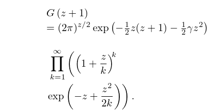
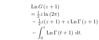
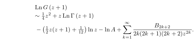
1: 5.17 Barnes’ $G$-Function (Double Gamma Function)

§5.17 Barnes’ $G$-Function (Double Gamma Function)

… ►

5.17.2 $$G\left(n\right)=(n-2)!(n-3)!\mathrm{\cdots }1!,$$ $n=2,3,\mathrm{\dots }$.

ⓘ

Symbols:

$G\left(z\right)$: Barnes’ $G$-function (or double gamma function), $!$: factorial (as in $n!$) and $n$: nonnegative integer

Permalink:

http://dlmf.nist.gov/5.17.E2

Encodings:

pMML, png, TeX

See also:

Annotations for §5.17 and Ch.5

►

5.17.3 $$G\left(z+1\right)={(2\pi )}^{z/2}\exp \left(-\frac{1}{2}z(z+1)-\frac{1}{2}\gamma z^2\right)\prod _{k=1}^{\mathrm{\infty }}\left({\left(1+\frac{z}{k}\right)}^k\exp \left(-z+\frac{z^2}{2k}\right)\right).$$

ⓘ

Symbols:

$G\left(z\right)$: Barnes’ $G$-function (or double gamma function), $\gamma$: Euler’s constant, $\pi$: the ratio of the circumference of a circle to its diameter, $\exp z$: exponential function, $k$: nonnegative integer and $z$: complex variable

Permalink:

http://dlmf.nist.gov/5.17.E3

Encodings:

pMML, png, TeX

See also:

Annotations for §5.17 and Ch.5

►

5.17.4 $$\mathrm{Ln}G\left(z+1\right)=\frac{1}{2}z\ln \left(2\pi \right)-\frac{1}{2}z(z+1)+z\mathrm{Ln}\mathrm{\Gamma }\left(z+1\right)-{\int }_0^z\mathrm{Ln}\mathrm{\Gamma }\left(t+1\right)dt.$$

ⓘ

Symbols:

$G\left(z\right)$: Barnes’ $G$-function (or double gamma function), $\mathrm{\Gamma }\left(z\right)$: gamma function, $\pi$: the ratio of the circumference of a circle to its diameter, $dx$: differential of $x$ , $\int$: integral, $\mathrm{Ln}z$: general logarithm function, $\ln z$: principal branch of logarithm function and $z$: complex variable

Permalink:

http://dlmf.nist.gov/5.17.E4

Encodings:

pMML, png, TeX

See also:

Annotations for §5.17 and Ch.5

… ►

5.17.5 $$\mathrm{Ln}G\left(z+1\right)\sim \frac{1}{4}{z}^2+z\mathrm{Ln}\mathrm{\Gamma }\left(z+1\right)-\left(\frac{1}{2}z(z+1)+\frac{1}{12}\right)\ln z-\ln A+\sum _{k=1}^{\mathrm{\infty }}\frac{B_{2k+2}}{2k(2k+1)(2k+2)z^{2k}}.$$

ⓘ

Symbols:

$G\left(z\right)$: Barnes’ $G$-function (or double gamma function), $B_n$: Bernoulli numbers, $\mathrm{\Gamma }\left(z\right)$: gamma function, $\sim$: Poincaré asymptotic expansion, $\mathrm{Ln}z$: general logarithm function, $\ln z$: principal branch of logarithm function, $k$: nonnegative integer, $z$: complex variable and $A$: Glaisher’s constant

Referenced by:

§5.17, §5.17, Erratum (V1.0.7) for Equation (5.17.5), Erratum (V1.1.11) for Equation (5.17.5)

Permalink:

http://dlmf.nist.gov/5.17.E5

Encodings:

pMML, png, TeX

Errata (effective with 1.1.11):

For consistency we have replaced $\mathrm{Ln}z$ by $\ln z$.

Errata (effective with 1.0.7):

Originally the term $z\mathrm{Ln}\mathrm{\Gamma }\left(z+1\right)$ was incorrectly stated as $z\mathrm{\Gamma }\left(z+1\right)$. (This error was reported subsequently by Nick Jones on December 11, 2013.)

Reported 2013-08-01 by Gergő Nemes

See also:

Annotations for §5.17 and Ch.5

…

2: 5.1 Special Notation

… ►

3: Bibliography F

… ►

ⓘ

Notes:

The “Freely Distributable LIBM” package provides implementations of standard elementary functions plus a few higher functions, e.g. gamma. Double precision, maximum accuracy 20S. Developed by Sun Microsystems.

External Links:

GAMS (package FDLIBM)

Referenced by:

§ ‣ Software Cross Index, § ‣ Software Cross Index.

Encodings:

BibTeX

… ►

An asymptotic expansion of the double gamma function. J. Approx. Theory 111 (2), pp. 298–314.

ⓘ

External Links:

ISSN 0021-9045, Document, MathReview (C. M. Joshi), ZentralBlatt

Referenced by:

§5.17.

Encodings:

BibTeX

…

4: Bibliography M

… ►

Further improvements of some double inequalities for bounding the gamma function. Math. Comput. Modelling 57 (5-6), pp. 1360–1363.

ⓘ

External Links:

ISSN 0895-7177, Document, FullText, MathReview (Emil C. Popa)

Referenced by:

§5.6(i).

Encodings:

BibTeX

…

5: 5.4 Special Values and Extrema

… ►

5.4.2

ⓘ

Symbols:

$\mathrm{\Gamma }\left(z\right)$: gamma function, $\pi$: the ratio of the circumference of a circle to its diameter, $!!$: double factorial and $n$: nonnegative integer

Referenced by:

§5.4(i), §5.4(i)

Permalink:

http://dlmf.nist.gov/5.4.E2

Encodings:

pMML, png, TeX

See also:

Annotations for §5.4(i), §5.4 and Ch.5

…

6: Bibliography Q

… ►

Some inequalities of the incomplete gamma and related functions. Z. Anal. Anwendungen 18 (3), pp. 793–799.

ⓘ

External Links:

ISSN 0232-2064, FullText, MathReview (Richard B. Paris), ZentralBlatt

Referenced by:

§8.10.

Encodings:

BibTeX

►

A new lower bound in the second Kershaw’s double inequality. J. Comput. Appl. Math. 214 (2), pp. 610–616.

ⓘ

External Links:

ISSN 0377-0427, Document, FullText, MathReview (Mehdi Hassani), ZentralBlatt

Referenced by:

§5.6(i), §5.6(i).

Encodings:

BibTeX

… ►

Uniform asymptotic expansions of a double integral: Coalescence of two stationary points. Proc. Roy. Soc. London Ser. A 456, pp. 407–431.

ⓘ

External Links:

ISSN 1364-5021, Document, MathReview (F. Ursell), ZentralBlatt

Referenced by:

§2.4(vi).

Encodings:

BibTeX

… ►

“Best possible” upper and lower bounds for the zeros of the Bessel function $J_{\nu }(x)$ . Trans. Amer. Math. Soc. 351 (7), pp. 2833–2859.

ⓘ

External Links:

ISSN 0002-9947, FullText, MathReview (Andrea Laforgia), ZentralBlatt

Referenced by:

§10.21(vii).

Encodings:

BibTeX

…

7: 8.13 Zeros

§8.13 Zeros

… ►The function ${\gamma }^{\ast }(a,x)$ has no real zeros for $a\ge 0$. … ►When $-5\le a\le 4$ the behavior of the $x$-zeros as functions of $a$ can be seen by taking the slice ${\gamma }^{\ast }(a,x)=0$ of the surface depicted in Figure 8.3.6. … ►As $x$ increases the positive zeros coalesce to form a double zero at ($a_n^{\ast },x_n^{\ast }$). The values of the first six double zeros are given to 5D in Table 8.13.1. …

8: 21.5 Modular Transformations

… ►

21.5.5

ⓘ

Symbols:

$\theta \left(𝐳\right|𝛀)$: Riemann theta function, ${𝐀}^{\mathrm{T}}$: transpose of matrix, $g$: positive integer, $𝛀$: a Riemann matrix and Matrix $𝚪$

Permalink:

http://dlmf.nist.gov/21.5.E5

Encodings:

pMML, png, TeX

See also:

Annotations for §21.5(i), §21.5 and Ch.21

… ►

21.5.6

ⓘ

Symbols:

$\theta \left(𝐳\right|𝛀)$: Riemann theta function, $g$: positive integer, $𝛀$: a Riemann matrix and Matrix $𝚪$

Permalink:

http://dlmf.nist.gov/21.5.E6

Encodings:

pMML, png, TeX

See also:

Annotations for §21.5(i), §21.5 and Ch.21

… ►

21.5.7

ⓘ

Symbols:

$\theta \left(𝐳\right|𝛀)$: Riemann theta function, $g$: positive integer, $𝛀$: a Riemann matrix, $\mathrm{diag}𝐀$: Transpose of $[A_{11},A_{22},\mathrm{\dots },A_{gg}]$ and Matrix $𝚪$

Referenced by:

(21.5.8), Erratum (V1.0.11) for Clarifications

Permalink:

http://dlmf.nist.gov/21.5.E7

Encodings:

pMML, png, TeX

See also:

Annotations for §21.5(i), §21.5 and Ch.21

…

9: 16.15 Integral Representations and Integrals

… ►

16.15.3 $$F_3(\alpha ,{\alpha }^{\prime };\beta ,{\beta }^{\prime };\gamma ;x,y)=\frac{\mathrm{\Gamma }\left(\gamma \right)}{\mathrm{\Gamma }\left(\beta \right)\mathrm{\Gamma }\left({\beta }^{\prime }\right)\mathrm{\Gamma }\left(\gamma -\beta -{\beta }^{\prime }\right)}{\iint }_{\mathrm{\Delta }}\frac{u^{\beta -1}{v}^{{\beta }^{\prime }-1}{(1-u-v)}^{\gamma -\beta -{\beta }^{\prime }-1}}{{(1-ux)}^{\alpha }{(1-vy)}^{{\alpha }^{\prime }}}dudv,$$ $\mathrm{\Re }\left(\gamma -\beta -{\beta }^{\prime }\right)>0$, $\mathrm{\Re }\beta >0$, $\mathrm{\Re }{\beta }^{\prime }>0$,

ⓘ

Symbols:

$F_3(\alpha ,{\alpha }^{\prime };\beta ,{\beta }^{\prime };\gamma ;x,y)$: third Appell function, $\mathrm{\Gamma }\left(z\right)$: gamma function, $dx$: differential of $x$ and $\mathrm{\Re }$: real part

Keywords:

Mellin transform

Notes:

Erdélyi et al. (1953a, 5.8.1(3)) contains a typo.

Referenced by:

Erratum (V1.0.14) for Equation (16.15.3), Erratum (V1.0.14) for Equation (16.15.3)

Permalink:

http://dlmf.nist.gov/16.15.E3

Encodings:

pMML, png, TeX

Clarification (effective with 1.0.14):

A stray “$f$” was removed; it appeared after the comma at the end of this equation.

See also:

Annotations for §16.15 and Ch.16

…

10: 15.6 Integral Representations

§15.6 Integral Representations

… ►In (15.6.1) all functions in the integrand assume their principal values. … ►In (15.6.6) the integration contour separates the poles of $\mathrm{\Gamma }\left(a+t\right)$ and $\mathrm{\Gamma }\left(b+t\right)$ from those of $\mathrm{\Gamma }\left(-t\right)$, and ${(-z)}^t$ has its principal value. ►In (15.6.7) the integration contour separates the poles of $\mathrm{\Gamma }\left(a+t\right)$ and $\mathrm{\Gamma }\left(b+t\right)$ from those of $\mathrm{\Gamma }\left(c-a-b-t\right)$ and $\mathrm{\Gamma }\left(-t\right)$, and ${(1-z)}^t$ has its principal value. ►In each of (15.6.8) and (15.6.9) all functions in the integrand assume their principal values. …