dominant solutions

SearchAdvancedHelp

(0.001 seconds)

9 matching pages

1: 2.9 Difference Equations

… ►As in the case of differential equations (§§2.7(iii), 2.7(iv)) recessive solutions are unique and dominant solutions are not; furthermore, one member of a numerically satisfactory pair has to be recessive. When $|{\rho }_2|=|{\rho }_1|$ and $\mathrm{\Re }{\alpha }_2=\mathrm{\Re }{\alpha }_1$ neither solution is dominant and both are unique. …

2: 2.7 Differential Equations

… ►

2.7.30 $$w_1(x)/w_4(x)\to 0,$$ $x\to a_1+$,

ⓘ

Symbols:

$(a_1,a_2)$: interval and $w_j(z)$: solutions

Permalink:

http://dlmf.nist.gov/2.7.E30

Encodings:

pMML, png, TeX

See also:

Annotations for §2.7(iii), §2.7(iii), §2.7 and Ch.2

► $w_1(x)$ is a recessive (or subdominant) solution as $x\to a_1+$, and $w_4(x)$ is a dominant solution as $x\to a_1+$. … ►The solutions $w_1(z)$ and $w_2(z)$ are respectively recessive and dominant as $\mathrm{\Re }z\to -\mathrm{\infty }$, and vice versa as $\mathrm{\Re }z\to +\mathrm{\infty }$. …

3: 18.39 Applications in the Physical Sciences

… ►The solutions of (18.39.8) are subject to boundary conditions at $a$ and $b$. … ►The solutions (18.39.8) are called the stationary states as separation of variables in (18.39.9) yields solutions of form … ►Brief mention of non-unit normalized solutions in the case of mixed spectra appear, but as these solutions are not OP’s details appear elsewhere, as referenced. … ►Interactions between electrons, in many electron atoms, breaks this degeneracy as a function of $l$, but $n$ still dominates. … ►The radial Coulomb wave functions $R_{n,l}(r)$, solutions of …

4: 36.5 Stokes Sets

… ►The Stokes sets are defined by the exponential dominance condition: … ►For , there are two solutions $u$, provided that $|Y|>{(\frac{2}{5})}^{1/2}$. … ►The first sheet corresponds to and is generated as a solution of Equations (36.5.6)–(36.5.9). …For $\left|Y\right|>Y_1$ the second sheet is generated by a second solution of (36.5.6)–(36.5.9), and for it is generated by the roots of the polynomial equation …

5: 36.11 Leading-Order Asymptotics

… ►

36.11.1

ⓘ

Symbols:

$t_j(𝐱)$: solutions

Permalink:

http://dlmf.nist.gov/36.11.E1

Encodings:

pMML, png, TeX

See also:

Annotations for §36.11 and Ch.36

… ►

36.11.2 $${\mathrm{\Psi }}_K\left(𝐱\right)=\sqrt{2\pi }\sum _{j=1}^{j_{\max }(𝐱)}\exp \left(\mathrm{i}\left({\mathrm{\Phi }}_K(t_j(𝐱);𝐱)+\frac{1}{4}\pi {(-1)}^{j+K+1}\right)\right){\left|\frac{{\partial }^2{\mathrm{\Phi }}_K(t_j(𝐱);𝐱)}{{\partial t}^2}\right|}^{-1/2}(1+o\left(1\right)).$$

ⓘ

Symbols:

${\mathrm{\Psi }}_K\left(𝐱\right)$: canonical integral function, $\pi$: the ratio of the circumference of a circle to its diameter, ${\mathrm{\Phi }}_K(t;𝐱)$: cuspoid catastrophe of codimension $K$ , $\exp z$: exponential function, $\mathrm{i}$: imaginary unit, $o\left(x\right)$: order less than, $\frac{\partial f}{\partial x}$: partial derivative of $f$ with respect to $x$ , $\partial x$: partial differential of $x$ , $t$: variable, $K$: codimension and $t_j(𝐱)$: solutions

Permalink:

http://dlmf.nist.gov/36.11.E2

Encodings:

pMML, png, TeX

See also:

Annotations for §36.11 and Ch.36

…

6: 2.11 Remainder Terms; Stokes Phenomenon

… ►In effect, (2.11.7) “corrects” (2.11.6) by introducing a term that is relatively exponentially small in the neighborhood of $\mathrm{ph}z=\pi$, is increasingly significant as $\mathrm{ph}z$ passes from $\pi$ to $\frac{3}{2}\pi$, and becomes the dominant contribution after $\mathrm{ph}z$ passes $\frac{3}{2}\pi$. … ►Rays (or curves) on which one contribution in a compound asymptotic expansion achieves maximum dominance over another are called Stokes lines ($\theta =\pi$ in the present example). … ►

§2.11(v) Exponentially-Improved Expansions (continued)

… ►

2.11.19 $$w_j(z)={\mathrm{e}}^{{\lambda }_{j}z}{z}^{{\mu }_j}\sum _{s=0}^{n-1}\frac{a_{s,j}}{z^s}+R_n^{(j)}(z),$$ $j=1,2$,

ⓘ

Symbols:

$\mathrm{e}$: base of natural logarithm, $R_n^{(j)}(z)$: remainder, $a_{s,j}$: coefficients, ${\lambda }_j$: roots, ${\mu }_j$: quantities and $w_j(z)$: solutions

Permalink:

http://dlmf.nist.gov/2.11.E19

Encodings:

pMML, png, TeX

See also:

Annotations for §2.11(v), §2.11 and Ch.2

…

7: 3.6 Linear Difference Equations

§3.6 Linear Difference Equations

… ►

§3.6(ii) Homogeneous Equations

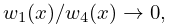
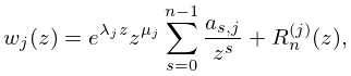
… ► … ► … ►Thus $Y_n\left(1\right)$ is dominant and can be computed by forward recursion, whereas $J_n\left(1\right)$ is recessive and has to be computed by backward recursion. …

8: Bibliography H

… ►

Asymptotic expansion of a class of integral transforms with algebraically dominated kernels. J. Math. Anal. Appl. 35 (2), pp. 405–433.

ⓘ

External Links:

Document, MathReview (E. L. Koh), ZentralBlatt

Referenced by:

§2.5(ii).

Encodings:

BibTeX

… ►

High frequency solutions of the delta wing equations. Proc. Roy. Soc. Edinburgh Sect. A 81 (3-4), pp. 299–316.

ⓘ

External Links:

ISSN 0308-2105, MathReview (V. M. Babich), ZentralBlatt

Referenced by:

§29.19(ii).

Encodings:

BibTeX

… ►

Numerical Tools for the Study of Finite Gap Solutions of Integrable Systems. Ph.D. Thesis, Technischen Universität Berlin.

ⓘ

Notes:

(All relevant material, plus corrections, are included in Deconinck et al. (2004).)

External Links:

ZentralBlatt

Referenced by:

§21.5(i).

Encodings:

BibTeX

… ►

Solutions of Poisson’s equation in channel-like geometries. Comput. Phys. Comm. 115 (1), pp. 45–68.

ⓘ

External Links:

ISSN 0010-4655, Document, Code, MathReview Entry, ZentralBlatt

Referenced by:

§14.31(i).

Encodings:

BibTeX

…

9: 1.2 Elementary Algebra

… ►Square $n\times n$ matrices (said to be of order $n$ ) dominate the use of matrices in the DLMF, and they have many special properties. … ►has a unique solution, $𝐛={𝐀}^{-1}𝐜$. If $det(𝐀)=0$ then, depending on $𝐜$, there is either no solution or there are infinitely many solutions, being the sum of a particular solution of (1.2.61) and any solution of $𝐀𝐛=𝟎$. Numerical methods and issues for solution of (1.2.61) appear in §§3.2(i) to 3.2(iii). … ►Numerical methods and issues for solution of (1.2.72) appear in §§3.2(iv) to 3.2(vii). …