differentiable functions
(0.003 seconds)
1—10 of 31 matching pages
1: 1.4 Calculus of One Variable
…
►If exists and is continuous on an interval , then we write .
…When is unbounded, is infinitely differentiable on and we write .
…
►
Mean Value Theorem
… ►If , then …2: 4.12 Generalized Logarithms and Exponentials
3: 2.8 Differential Equations with a Parameter
…
►in which ranges over a bounded or unbounded interval or domain , and is or analytic on .
…
►Again, and is on .
Corresponding to each positive integer there are solutions , , that are on , and as
…
►Also, is on , and .
…
►In the former, corresponding to any positive integer there are solutions , , that are on , and as
…
4: 3.5 Quadrature
…
►where , , and .
…
►If in addition is periodic, , and the integral is taken over a period, then
…
►Let and .
…
►If , then the remainder in (3.5.2) can be expanded in the form
…
►For
functions Gauss quadrature can be very efficient.
…
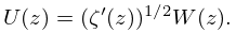
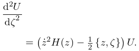
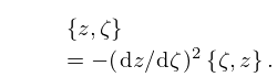
5: 1.13 Differential Equations
…
►Let satisfy (1.13.14), be any thrice-differentiable function of , and
►
1.13.18
…
►
1.13.19
…
►
1.13.22
…
►As the interval is mapped, one-to-one, onto by the above definition of , the integrand being positive, the inverse of this same transformation allows to be calculated from in (1.13.31), and .
…
6: 1.8 Fourier Series
…
►If a function
is periodic, with period , then the series obtained by differentiating the Fourier series for term by term converges at every point to .
…
7: 3.7 Ordinary Differential Equations
…
►If is on the closure of , then the discretized form (3.7.13) of the differential equation can be used.
…
8: 1.18 Linear Second Order Differential Operators and Eigenfunction Expansions
…
►and functions
, assumed real for the moment.
…
►For we can take , with appropriate boundary conditions, and with compact support if is bounded, which space is dense in , and for unbounded require that possible non- eigenfunctions of (1.18.28), with real eigenvalues, are non-zero but bounded on open intervals, including .
…
►, ) of which is moreover in .
…
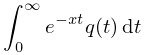
9: 2.3 Integrals of a Real Variable
…
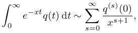
►
2.3.1
►converges for all sufficiently large , and is infinitely differentiable in a neighborhood of the origin.
…
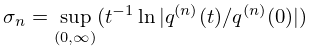
►
2.3.2
.
…
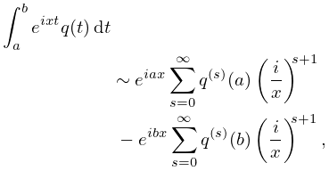
►
2.3.3
…
►
2.3.4
.
…
