determinants
(0.001 seconds)
1—10 of 34 matching pages
1: 1.3 Determinants, Linear Operators, and Spectral Expansions
…
►
§1.3(i) Determinants: Elementary Properties
… ►Relationships Between Determinants
… ►§1.3(ii) Special Determinants
… ►Vandermonde Determinant or Vandermondian
… ►Cauchy Determinant
…2: 24.14 Sums
…
►These identities can be regarded as higher-order recurrences.
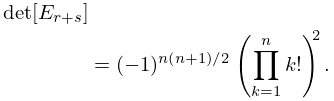
Let denote a Hankel (or persymmetric) determinant, that is, an
determinant with element in row and column for .
…
►
24.14.11
►
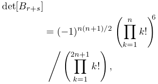
24.14.12
…
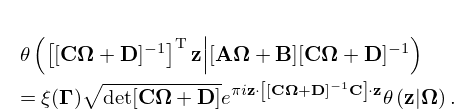
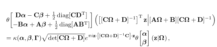
3: 21.5 Modular Transformations

4: 1.2 Elementary Algebra
…
►
The Determinant
►The matrix has a determinant, , explored further in §1.3, denoted, in full index form, as …where is defined by the Leibniz formula … ►A square matrix is singular if , otherwise it is non-singular. … ►Relation of Eigenvalues to the Determinant and Trace
…5: 1.1 Special Notation
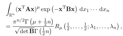
6: 19.31 Probability Distributions
…
►
19.31.2
.
…
7: 3.9 Acceleration of Convergence
…
►
3.9.9
,
►where is the Hankel determinant
►

3.9.10
►The ratio of the Hankel determinants in (3.9.9) can be computed recursively by Wynn’s epsilon algorithm:
…

8: 32.8 Rational Solutions
…
►
– possess hierarchies of rational solutions for special values of the parameters which are generated from “seed solutions” using the Bäcklund transformations and often can be expressed in the form of determinants.
…
►where is the Wronskian determinant
…
►For determinantal representations see Kajiwara and Masuda (1999).
…
►For determinantal representations see Kajiwara and Ohta (1998) and Noumi and Yamada (1999).
…
►For determinantal representations see Masuda et al. (2002).
…
9: 32.10 Special Function Solutions
…
►where is the Wronskian determinant
…
►For determinantal representations see Forrester and Witte (2002) and Okamoto (1987c).
…
►For determinantal representations see Forrester and Witte (2001) and Okamoto (1986).
…
►For determinantal representations see Forrester and Witte (2002), Masuda (2004), and Okamoto (1987b).
…
►For determinantal representations see Forrester and Witte (2004) and Masuda (2004).
…
