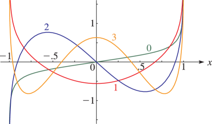
About the Project

cut

AdvancedHelp

(0.000 seconds)

1—10 of 66 matching pages

1: 30.5 Functions of the Second Kind
30.5.1 𝖰𝗌 n m ( x , γ 2 ) , n = m , m + 1 , m + 2 , .
30.5.2 𝖰𝗌 n m ( x , γ 2 ) = ( 1 ) n m + 1 𝖰𝗌 n m ( x , γ 2 ) ,
30.5.4 𝒲 { 𝖯𝗌 n m ( x , γ 2 ) , 𝖰𝗌 n m ( x , γ 2 ) } = ( n + m ) ! ( 1 x 2 ) ( n m ) ! A n m ( γ 2 ) A n m ( γ 2 ) ( 0 ) ,
2: 30.4 Functions of the First Kind
The eigenfunctions of (30.2.1) that correspond to the eigenvalues λ n m ( γ 2 ) are denoted by 𝖯𝗌 n m ( x , γ 2 ) , n = m , m + 1 , m + 2 , . …the sign of 𝖯𝗌 n m ( 0 , γ 2 ) being ( 1 ) ( n + m ) / 2 when n m is even, and the sign of d 𝖯𝗌 n m ( x , γ 2 ) / d x | x = 0 being ( 1 ) ( n + m 1 ) / 2 when n m is odd. When γ 2 > 0 𝖯𝗌 n m ( x , γ 2 ) is the prolate angular spheroidal wave function, and when γ 2 < 0 𝖯𝗌 n m ( x , γ 2 ) is the oblate angular spheroidal wave function. If γ = 0 , 𝖯𝗌 n m ( x , 0 ) reduces to the Ferrers function 𝖯 n m ( x ) : … 𝖯𝗌 n m ( x , γ 2 ) has exactly n m zeros in the interval 1 < x < 1 . …
3: 30.1 Special Notation
The main functions treated in this chapter are the eigenvalues λ n m ( γ 2 ) and the spheroidal wave functions 𝖯𝗌 n m ( x , γ 2 ) , 𝖰𝗌 n m ( x , γ 2 ) , 𝑃𝑠 n m ( z , γ 2 ) , 𝑄𝑠 n m ( z , γ 2 ) , and S n m ( j ) ( z , γ ) , j = 1 , 2 , 3 , 4 . …Meixner and Schäfke (1954) use ps , qs , Ps , Qs for 𝖯𝗌 , 𝖰𝗌 , 𝑃𝑠 , 𝑄𝑠 , respectively. … Flammer (1957) and Abramowitz and Stegun (1964) use λ m n ( γ ) for λ n m ( γ 2 ) + γ 2 , R m n ( j ) ( γ , z ) for S n m ( j ) ( z , γ ) , and
S m n ( 1 ) ( γ , x ) = d m n ( γ ) 𝖯𝗌 n m ( x , γ 2 ) ,
S m n ( 2 ) ( γ , x ) = d m n ( γ ) 𝖰𝗌 n m ( x , γ 2 ) ,
4: 30.7 Graphics
See accompanying text
Figure 30.7.5: 𝖯𝗌 n 0 ( x , 4 ) , n = 0 , 1 , 2 , 3 , 1 x 1 . Magnify
See accompanying text
Figure 30.7.6: 𝖯𝗌 n 0 ( x , 4 ) , n = 0 , 1 , 2 , 3 , 1 x 1 . Magnify
See accompanying text
Figure 30.7.7: 𝖯𝗌 n 1 ( x , 30 ) , n = 1 , 2 , 3 , 4 , 1 x 1 . Magnify
See accompanying text
Figure 30.7.8: 𝖯𝗌 n 1 ( x , 30 ) , n = 1 , 2 , 3 , 4 , 1 x 1 . Magnify
See accompanying text
Figure 30.7.11: 𝖰𝗌 n 0 ( x , 4 ) , n = 0 , 1 , 2 , 3 , 1 < x < 1 . Magnify
5: 14.22 Graphics
See accompanying text
Figure 14.22.1: P 1 / 2 0 ( x + i y ) , 5 x 5 , 5 y 5 . There is a cut along the real axis from to 1 . Magnify 3D Help
See accompanying text
Figure 14.22.2: P 1 / 2 1 / 2 ( x + i y ) , 5 x 5 , 5 y 5 . There is a cut along the real axis from to 1 . Magnify 3D Help
See accompanying text
Figure 14.22.3: P 1 / 2 1 ( x + i y ) , 5 x 5 , 5 y 5 . There is a cut along the real axis from to 1 . Magnify 3D Help
See accompanying text
Figure 14.22.4: 𝑸 0 0 ( x + i y ) , 5 x 5 , 5 y 5 . There is a cut along the real axis from 1 to 1 . Magnify 3D Help
6: 30.10 Series and Integrals
Integrals and integral equations for 𝖯𝗌 n m ( x , γ 2 ) are given in Arscott (1964b, §8.6), Erdélyi et al. (1955, §16.13), Flammer (1957, Chapter 5), and Meixner (1951). …
7: 4.37 Inverse Hyperbolic Functions
These functions are analytic in the cut plane depicted in Figure 4.37.1(iv), (v), (vi), respectively. …
§4.37(iv) Logarithmic Forms
On the cutsOn the part of the cuts from 1 to 1 On the cuts
8: 30.6 Functions of Complex Argument
9: 4.2 Definitions
Most texts extend the definition of the principal value to include the branch cut …where k is the excess of the number of times the path in (4.2.1) crosses the negative real axis in the positive sense over the number of times in the negative sense. In the DLMF we allow a further extension by regarding the cut as representing two sets of points, one set corresponding to the “upper side” and denoted by z = x + i 0 , the other set corresponding to the “lower side” and denoted by z = x i 0 . …Consequently ln z is two-valued on the cut, and discontinuous across the cut. … This is an analytic function of z on ( , 0 ] , and is two-valued and discontinuous on the cut shown in Figure 4.2.1, unless a . …
10: 4.39 Continued Fractions
where z is in the open cut plane of Figure 4.37.1(i). …where z is in the open cut plane of Figure 4.37.1(iii). …