conversions between variables and parameters

SearchAdvancedHelp

(0.004 seconds)

1—10 of 325 matching pages

1: 33.22 Particle Scattering and Atomic and Molecular Spectra

… ►

$𝗄$ Scaling

… ►

$Z$ Scaling

… ►

$\mathrm{i}𝗄$ Scaling

… ►

§33.22(iii) Conversions Between Variables

… ►

§33.22(vii) Complex Variables and Parameters

…

2: 28.27 Addition Theorems

… ►Addition theorems provide important connections between Mathieu functions with different parameters and in different coordinate systems. …

3: Bille C. Carlson

… ►In his paper Lauricella’s hypergeometric function $F_D$ (1963), he defined the $R$-function, a multivariate hypergeometric function that is homogeneous in its variables, each variable being paired with a parameter. If some of the parameters are equal, then the $R$-function is symmetric in the corresponding variables. …

4: 31.16 Mathematical Applications

… ►

31.16.1 $${\mathrm{𝐻𝑝}}_{n,m}\left(x\right){\mathrm{𝐻𝑝}}_{n,m}\left(y\right)=\sum _{j=0}^n{A}_j{\sin }^{2j}\theta P_{n-j}^{(\gamma +\delta +2j-1,ϵ-1)}\left(\cos \left(2\theta \right)\right)P_j^{(\delta -1,\gamma -1)}\left(\cos \left(2\varphi \right)\right),$$

ⓘ

Symbols:

${\mathrm{𝐻𝑝}}_{n,m}(a,q_{n,m};-n,\beta ,\gamma ,\delta ;z)$: Heun polynomials, $P_n^{(\alpha ,\beta )}\left(x\right)$: Jacobi polynomial, $\cos z$: cosine function, $\sin z$: sine function, $\gamma$: real or complex parameter, $\delta$: real or complex parameter, $ϵ$: real or complex parameter, $j$: nonnegative integer, $m$: nonnegative integer, $n$: nonnegative integer, $a$: complex parameter, $q$: real or complex parameter, $\beta$: real or complex parameter, $\theta$: angle, $\varphi$: angle, $x$: variable, $y$: variable and $A_j$: coefficients

Referenced by:

§31.16(ii), §31.16(ii)

Permalink:

http://dlmf.nist.gov/31.16.E1

Encodings:

pMML, png, TeX

See also:

Annotations for §31.16(ii), §31.16 and Ch.31

…

5: 32.6 Hamiltonian Structure

… ►Conversely, if $\sigma$ is a solution of (32.6.6), then … ►Conversely, if $\sigma (z)$ is a solution of (32.6.13), then … ►Conversely, if $\sigma$ is a solution of (32.6.21), then … ►Conversely, if $\sigma$ is a solution of (32.6.29), then … ►Conversely, if $\sigma$ is a solution of (32.6.37), then …

6: 28.29 Definitions and Basic Properties

… ►

28.29.1 $$w^{\prime \prime }(z)+\left(\lambda +Q(z)\right)w=0,$$

ⓘ

Symbols:

$z$: complex variable, $w(z)$: Mathieu’s equation solution, $\lambda$: parameter and $Q(z)$: function

Referenced by:

§28.29(ii), §28.29(ii), §28.29(ii), §28.29(iii), §28.29(iii), §28.29(iii)

Permalink:

http://dlmf.nist.gov/28.29.E1

Encodings:

pMML, png, TeX

See also:

Annotations for §28.29(i), §28.29 and Ch.28

… ►

28.29.7 $$w(z+\pi )={\mathrm{e}}^{\pi \mathrm{i}\nu }w(z),$$

ⓘ

Symbols:

$\pi$: the ratio of the circumference of a circle to its diameter, $\mathrm{e}$: base of natural logarithm, $\mathrm{i}$: imaginary unit, $z$: complex variable, $\nu$: complex parameter and $w(z)$: Mathieu’s equation solution

Referenced by:

§28.29(ii)

Permalink:

http://dlmf.nist.gov/28.29.E7

Encodings:

pMML, png, TeX

See also:

Annotations for §28.29(ii), §28.29 and Ch.28

… ►

28.29.10 $$F_{\nu }(z)={\mathrm{e}}^{\mathrm{i}\nu z}{P}_{\nu }(z),$$

ⓘ

Defines:

$F_{\nu }(z)$: Floquet solution (locally)

Symbols:

$\mathrm{e}$: base of natural logarithm, $\mathrm{i}$: imaginary unit, $z$: complex variable and $\nu$: complex parameter

Permalink:

http://dlmf.nist.gov/28.29.E10

Encodings:

pMML, png, TeX

See also:

Annotations for §28.29(ii), §28.29 and Ch.28

… ►

28.29.11 $$w(z+\pi )={(-1)}^{\nu }w(z)+cP(z),$$

ⓘ

Symbols:

$\pi$: the ratio of the circumference of a circle to its diameter, $z$: complex variable, $\nu$: complex parameter, $w(z)$: Mathieu’s equation solution and $c$: constant

Permalink:

http://dlmf.nist.gov/28.29.E11

Encodings:

pMML, png, TeX

See also:

Annotations for §28.29(ii), §28.29 and Ch.28

… ►

28.29.13 $$w(z+\pi )+w(z-\pi )=2\cos \left(\pi \nu \right)w(z).$$

ⓘ

Symbols:

$\pi$: the ratio of the circumference of a circle to its diameter, $\cos z$: cosine function, $z$: complex variable, $\nu$: complex parameter and $w(z)$: Mathieu’s equation solution

Permalink:

http://dlmf.nist.gov/28.29.E13

Encodings:

pMML, png, TeX

See also:

Annotations for §28.29(ii), §28.29 and Ch.28

…

7: 4.3 Graphics

… ►

►►

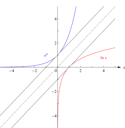
Figure 4.3.1: $\ln x$ and ${\mathrm{e}}^x$. Parallel tangent lines at $(1,0)$ and $(0,1)$ make evident the mirror symmetry across the line $y=x$, demonstrating the inverse relationship between the two functions. Magnify

… ►In the labeling of corresponding points $r$ is a real parameter that can lie anywhere in the interval $(0,\mathrm{\infty })$. …

8: 32.11 Asymptotic Approximations for Real Variables

§32.11 Asymptotic Approximations for Real Variables

… ►Conversely, for any nonzero real $k$, there is a unique solution $w_k(x)$ of (32.11.4) that is asymptotic to $k\mathrm{Ai}\left(x\right)$ as $x\to +\mathrm{\infty }$. … ►Conversely, for any $h$ $(\ne 0)$ there is a unique solution $w_h(x)$ of (32.11.29) that is asymptotic to $h{U}^2(-\nu -\frac{1}{2},\sqrt{2}x)$ as $x\to +\mathrm{\infty }$. … ►In terms of the parameter $k$ that is used in these figures $h=2^{3/2}{k}^2$. …

9: 28.2 Definitions and Basic Properties

… ►

28.2.1 $$w^{\prime \prime }+(a-2q\cos \left(2z\right))w=0.$$

ⓘ

Symbols:

$\cos z$: cosine function, $q=h^2$: parameter, $z$: complex variable, $a$: parameter and $w(z)$: Mathieu’s equation solution

A&S Ref:

20.3.1 20.1.1 (in slightly different form)

Referenced by:

§1.18(vii), Figure 28.17.1, Figure 28.17.1, §28.17, §28.17, §28.2(ii), §28.2(ii), §28.2(iii), §28.2(iv), §28.20(i), §28.29(i), §28.32(i), §28.32(i), 1st item, 2nd item, §28.33(iii), item (a), item (c), item (c), §28.5(i), §28.8(iv), §28.8(iv), §28.8(iv), §30.2(iii)

Permalink:

http://dlmf.nist.gov/28.2.E1

Encodings:

pMML, png, TeX

See also:

Annotations for §28.2(i), §28.2 and Ch.28

… ►

28.2.2 $$\zeta (1-\zeta )w^{\prime \prime }+\frac{1}{2}(1-2\zeta )w^{\prime }+\frac{1}{4}(a-2q(1-2\zeta ))w=0.$$

ⓘ

Symbols:

$q=h^2$: parameter, $a$: parameter, $w(z)$: Mathieu’s equation solution and $\zeta$: change of variable

Permalink:

http://dlmf.nist.gov/28.2.E2

Encodings:

pMML, png, TeX

See also:

Annotations for §28.2(i), §28.2 and Ch.28

… ►

28.2.3 $$(1-{\zeta }^2)w^{\prime \prime }-\zeta w^{\prime }+\left(a+2q-4q{\zeta }^2\right)w=0.$$

ⓘ

Symbols:

$q=h^2$: parameter, $a$: parameter, $w(z)$: Mathieu’s equation solution and $\zeta$: change of variable

A&S Ref:

20.1.7 (in slightly different notation)

Permalink:

http://dlmf.nist.gov/28.2.E3

Encodings:

pMML, png, TeX

See also:

Annotations for §28.2(i), §28.2 and Ch.28

… ►

28.2.7 $$w_{\text{I}}(z\pm \pi ;a,q)=w_{\text{I}}(\pi ;a,q)w_{\text{I}}(z;a,q)\pm w_{\text{I}}^{\prime }(\pi ;a,q)w_{\text{II}}(z;a,q),$$

ⓘ

Symbols:

$\pi$: the ratio of the circumference of a circle to its diameter, $q=h^2$: parameter, $z$: complex variable, $a$: parameter, $w(z)$: Mathieu’s equation solution, $w_{\text{I}}(z;a,q)$: fundamental solution and $w_{\text{II}}(z;a,q)$: fundamental solution

Referenced by:

§28.2(iv)

Permalink:

http://dlmf.nist.gov/28.2.E7

Encodings:

pMML, png, TeX

See also:

Annotations for §28.2(ii), §28.2 and Ch.28

►

28.2.8 $$w_{\text{II}}(z\pm \pi ;a,q)=\pm w_{\text{II}}(\pi ;a,q)w_{\text{I}}(z;a,q)+w_{\text{II}}^{\prime }(\pi ;a,q)w_{\text{II}}(z;a,q),$$

ⓘ

Symbols:

$\pi$: the ratio of the circumference of a circle to its diameter, $q=h^2$: parameter, $z$: complex variable, $a$: parameter, $w(z)$: Mathieu’s equation solution, $w_{\text{I}}(z;a,q)$: fundamental solution and $w_{\text{II}}(z;a,q)$: fundamental solution

Permalink:

http://dlmf.nist.gov/28.2.E8

Encodings:

pMML, png, TeX

See also:

Annotations for §28.2(ii), §28.2 and Ch.28

…

10: 31.3 Basic Solutions

… ►

31.3.5 $$z^{1-\gamma }H\mathrm{\ell }(a,(a\delta +ϵ)(1-\gamma )+q;\alpha +1-\gamma ,\beta +1-\gamma ,2-\gamma ,\delta ;z).$$

ⓘ

Symbols:

$H\mathrm{\ell }(a,q;\alpha ,\beta ,\gamma ,\delta ;z)$: Heun functions, $z$: complex variable, $\gamma$: real or complex parameter, $\delta$: real or complex parameter, $ϵ$: real or complex parameter, $a$: complex parameter, $q$: real or complex parameter, $\alpha$: real or complex parameter and $\beta$: real or complex parameter

Referenced by:

§31.3(iii), §31.7(ii)

Permalink:

http://dlmf.nist.gov/31.3.E5

Encodings:

pMML, png, TeX

See also:

Annotations for §31.3(i), §31.3 and Ch.31

… ►

31.3.6 $$H\mathrm{\ell }(1-a,\alpha \beta -q;\alpha ,\beta ,\delta ,\gamma ;1-z),$$

ⓘ

Symbols:

$H\mathrm{\ell }(a,q;\alpha ,\beta ,\gamma ,\delta ;z)$: Heun functions, $z$: complex variable, $\gamma$: real or complex parameter, $\delta$: real or complex parameter, $a$: complex parameter, $q$: real or complex parameter, $\alpha$: real or complex parameter and $\beta$: real or complex parameter

Permalink:

http://dlmf.nist.gov/31.3.E6

Encodings:

pMML, png, TeX

See also:

Annotations for §31.3(ii), §31.3 and Ch.31

►

31.3.7 $${(1-z)}^{1-\delta }H\mathrm{\ell }(1-a,((1-a)\gamma +ϵ)(1-\delta )+\alpha \beta -q;\alpha +1-\delta ,\beta +1-\delta ,2-\delta ,\gamma ;1-z).$$

ⓘ

Symbols:

$H\mathrm{\ell }(a,q;\alpha ,\beta ,\gamma ,\delta ;z)$: Heun functions, $z$: complex variable, $\gamma$: real or complex parameter, $\delta$: real or complex parameter, $ϵ$: real or complex parameter, $a$: complex parameter, $q$: real or complex parameter, $\alpha$: real or complex parameter and $\beta$: real or complex parameter

Permalink:

http://dlmf.nist.gov/31.3.E7

Encodings:

pMML, png, TeX

See also:

Annotations for §31.3(ii), §31.3 and Ch.31

… ►

31.3.8 $$H\mathrm{\ell }(\frac{a}{a-1},\frac{\alpha \beta a-q}{a-1};\alpha ,\beta ,ϵ,\delta ;\frac{a-z}{a-1}),$$

ⓘ

Symbols:

$H\mathrm{\ell }(a,q;\alpha ,\beta ,\gamma ,\delta ;z)$: Heun functions, $z$: complex variable, $\delta$: real or complex parameter, $ϵ$: real or complex parameter, $a$: complex parameter, $q$: real or complex parameter, $\alpha$: real or complex parameter and $\beta$: real or complex parameter

Permalink:

http://dlmf.nist.gov/31.3.E8

Encodings:

pMML, png, TeX

See also:

Annotations for §31.3(ii), §31.3 and Ch.31

… ►

31.3.12 $$H\mathrm{\ell }(1/a,q/a;\alpha ,\beta ,\gamma ,\alpha +\beta +1-\gamma -\delta ;z/a),$$

ⓘ

Symbols:

$H\mathrm{\ell }(a,q;\alpha ,\beta ,\gamma ,\delta ;z)$: Heun functions, $z$: complex variable, $\gamma$: real or complex parameter, $\delta$: real or complex parameter, $a$: complex parameter, $q$: real or complex parameter, $\alpha$: real or complex parameter and $\beta$: real or complex parameter

Permalink:

http://dlmf.nist.gov/31.3.E12

Encodings:

pMML, png, TeX

See also:

Annotations for §31.3(iii), §31.3 and Ch.31

…