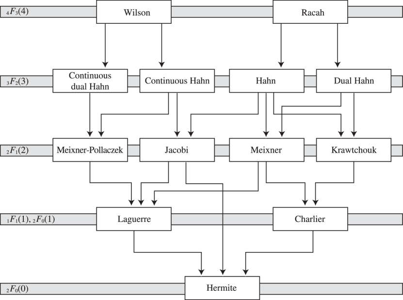
About the Project

continuous Hahn polynomials

AdvancedHelp

(0.004 seconds)

1—10 of 13 matching pages

1: 18.20 Hahn Class: Explicit Representations
18.20.3 w ( x ; a , b , a ¯ , b ¯ ) p n ( x ; a , b , a ¯ , b ¯ ) = 1 n ! δ x n ( w ( x ; a + 1 2 n , b + 1 2 n , a ¯ + 1 2 n , b ¯ + 1 2 n ) ) .
(For symmetry properties of p n ( x ; a , b , a ¯ , b ¯ ) with respect to a , b , a ¯ , b ¯ see Andrews et al. (1999, Corollary 3.3.4).) …
2: 18.22 Hahn Class: Recurrence Relations and Differences
18.22.4 q n ( x ) = p n ( x ; a , b , a ¯ , b ¯ ) / p n ( i a ; a , b , a ¯ , b ¯ ) ,
18.22.27 δ x ( p n ( x ; a , b , a ¯ , b ¯ ) ) = ( n + 2 ( a + b ) 1 ) p n 1 ( x ; a + 1 2 , b + 1 2 , a ¯ + 1 2 , b ¯ + 1 2 ) ,
3: 18.19 Hahn Class: Definitions
18.19.1 p n ( x ) = p n ( x ; a , b , a ¯ , b ¯ ) ,
4: 18.21 Hahn Class: Interrelations
18.21.10 lim t t n p n ( x t ; λ + i t , t tan ϕ , λ i t , t tan ϕ ) = ( 1 ) n ( cos ϕ ) n P n ( λ ) ( x ; ϕ ) .
See accompanying text
Figure 18.21.1: Askey scheme. …(This is with the convention that the real and imaginary parts of the parameters are counted separately in the case of the continuous Hahn polynomials.) Magnify
5: 18.23 Hahn Class: Generating Functions
18.23.6 F 1 1 ( a + i x 2 a ; i z ) F 1 1 ( b ¯ i x 2 b ; i z ) = n = 0 p n ( x ; a , b , a ¯ , b ¯ ) ( 2 a ) n ( 2 b ) n z n .
6: 18.1 Notation
( z 1 , , z k ; q ) = ( z 1 ; q ) ( z k ; q ) .
  • Continuous Hahn: p n ( x ; a , b , a ¯ , b ¯ ) .

  • 7: 18.26 Wilson Class: Continued
    18.26.5 lim d W n ( x ; a , b , c , d ) ( a + d ) n = S n ( x ; a , b , c ) .
    18.26.6 lim t W n ( ( x + t ) 2 ; a i t , b i t , a ¯ + i t , b ¯ + i t ) ( 2 t ) n n ! = p n ( x ; a , b , a ¯ , b ¯ ) .
    18.26.8 lim t S n ( ( x t ) 2 ; λ + i t , λ i t , t cot ϕ ) / t n = n ! ( csc ϕ ) n P n ( λ ) ( x ; ϕ ) .
    18.26.15 δ y ( S n ( y 2 ; a , b , c ) ) / δ y ( y 2 ) = n S n 1 ( y 2 ; a + 1 2 , b + 1 2 , c + 1 2 ) .
    8: 18.25 Wilson Class: Definitions
    Table 18.25.1 lists the transformations of variable, orthogonality ranges, and parameter constraints that are needed in §18.2(i) for the Wilson polynomials W n ( x ; a , b , c , d ) , continuous dual Hahn polynomials S n ( x ; a , b , c ) , Racah polynomials R n ( x ; α , β , γ , δ ) , and dual Hahn polynomials R n ( x ; γ , δ , N ) .
    Table 18.25.1: Wilson class OP’s: transformations of variable, orthogonality ranges, and parameter constraints.
    OP p n ( x ) x = λ ( y ) Orthogonality range for y Constraints
    continuous dual Hahn S n ( x ; a , b , c ) y 2 ( 0 , ) ( a , b , c ) > 0 ; nonreal parameters in conjugate pairs
    Under certain conditions on their parameters the orthogonality range for the Wilson polynomials and continuous dual Hahn polynomials is ( 0 , ) S , where S is a specific finite set, e. …
    18.25.6 p n ( x ) = S n ( x ; a 1 , a 2 , a 3 ) ,
    Table 18.25.2 provides the leading coefficients k n 18.2(iii)) for the Wilson, continuous dual Hahn, Racah, and dual Hahn polynomials. …
    9: Bibliography
  • R. Askey (1985) Continuous Hahn polynomials. J. Phys. A 18 (16), pp. L1017–L1019.
  • 10: 18.2 General Orthogonal Polynomials
    This happens, for example, with the continuous Hahn polynomials and Meixner–Pollaczek polynomials18.20(i)). …