About the Project

constants

AdvancedHelp

(0.001 seconds)

1—10 of 435 matching pages

1: 3.12 Mathematical Constants
§3.12 Mathematical Constants
The fundamental constant …Other constants that appear in the DLMF include the base e of natural logarithms …see §4.2(ii), and Euler’s constant γ For access to online high-precision numerical values of mathematical constants see Sloane (2003). …
2: 30.1 Special Notation
x real variable. Except in §§30.7(iv), 30.11(ii), 30.13, and 30.14, 1 < x < 1 .
δ arbitrary small positive constant.
The main functions treated in this chapter are the eigenvalues λ n m ( γ 2 ) and the spheroidal wave functions 𝖯𝗌 n m ( x , γ 2 ) , 𝖰𝗌 n m ( x , γ 2 ) , 𝑃𝑠 n m ( z , γ 2 ) , 𝑄𝑠 n m ( z , γ 2 ) , and S n m ( j ) ( z , γ ) , j = 1 , 2 , 3 , 4 . …Meixner and Schäfke (1954) use ps , qs , Ps , Qs for 𝖯𝗌 , 𝖰𝗌 , 𝑃𝑠 , 𝑄𝑠 , respectively. … Flammer (1957) and Abramowitz and Stegun (1964) use λ m n ( γ ) for λ n m ( γ 2 ) + γ 2 , R m n ( j ) ( γ , z ) for S n m ( j ) ( z , γ ) , and …where d m n ( γ ) is a normalization constant determined by …
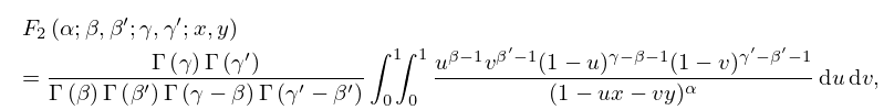
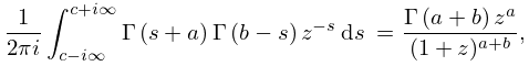
3: 16.15 Integral Representations and Integrals
16.15.1 F 1 ( α ; β , β ; γ ; x , y ) = Γ ( γ ) Γ ( α ) Γ ( γ α ) 0 1 u α 1 ( 1 u ) γ α 1 ( 1 u x ) β ( 1 u y ) β d u , α > 0 , ( γ α ) > 0 ,
16.15.2 F 2 ( α ; β , β ; γ , γ ; x , y ) = Γ ( γ ) Γ ( γ ) Γ ( β ) Γ ( β ) Γ ( γ β ) Γ ( γ β ) 0 1 0 1 u β 1 v β 1 ( 1 u ) γ β 1 ( 1 v ) γ β 1 ( 1 u x v y ) α d u d v , γ > β > 0 , γ > β > 0 ,
16.15.3 F 3 ( α , α ; β , β ; γ ; x , y ) = Γ ( γ ) Γ ( β ) Γ ( β ) Γ ( γ β β ) Δ u β 1 v β 1 ( 1 u v ) γ β β 1 ( 1 u x ) α ( 1 v y ) α d u d v , ( γ β β ) > 0 , β > 0 , β > 0 ,
16.15.4 F 4 ( α , β ; γ , γ ; x ( 1 y ) , y ( 1 x ) ) = Γ ( γ ) Γ ( γ ) Γ ( α ) Γ ( β ) Γ ( γ α ) Γ ( γ β ) 0 1 0 1 u α 1 v β 1 ( 1 u ) γ α 1 ( 1 v ) γ β 1 ( 1 u x ) γ + γ α 1 ( 1 v y ) γ + γ β 1 ( 1 u x v y ) α + β γ γ + 1 d u d v , γ > α > 0 , γ > β > 0 .
4: 32.9 Other Elementary Solutions
with κ , λ , μ , and ν arbitrary constants. … with C an arbitrary constant, which is solvable by quadrature. … with κ and μ arbitrary constants. … with C an arbitrary constant, which is solvable by quadrature. … with κ and μ arbitrary constants. …
5: 5.17 Barnes’ G -Function (Double Gamma Function)
G ( z + 1 ) = Γ ( z ) G ( z ) ,
Here B 2 k + 2 is the Bernoulli number (§24.2(i)), and A is Glaisher’s constant, given by
5.17.6 A = e C = 1.28242 71291 00622 63687 ,
5.17.7 C = lim n ( k = 1 n k ln k ( 1 2 n 2 + 1 2 n + 1 12 ) ln n + 1 4 n 2 ) = γ + ln ( 2 π ) 12 ζ ( 2 ) 2 π 2 = 1 12 ζ ( 1 ) ,
For Glaisher’s constant see also Greene and Knuth (1982, p. 100) and §2.10(i).
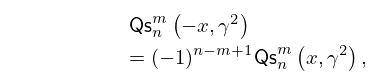
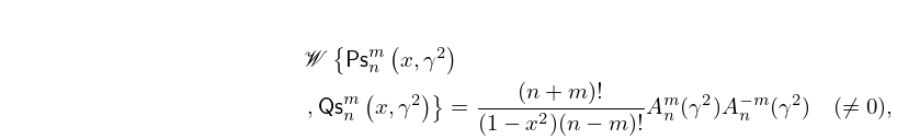
6: 30.5 Functions of the Second Kind
Other solutions of (30.2.1) with μ = m , λ = λ n m ( γ 2 ) , and z = x are
30.5.1 𝖰𝗌 n m ( x , γ 2 ) , n = m , m + 1 , m + 2 , .
30.5.2 𝖰𝗌 n m ( x , γ 2 ) = ( 1 ) n m + 1 𝖰𝗌 n m ( x , γ 2 ) ,
30.5.4 𝒲 { 𝖯𝗌 n m ( x , γ 2 ) , 𝖰𝗌 n m ( x , γ 2 ) } = ( n + m ) ! ( 1 x 2 ) ( n m ) ! A n m ( γ 2 ) A n m ( γ 2 ) ( 0 ) ,
with A n ± m ( γ 2 ) as in (30.11.4). …
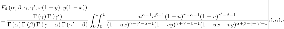
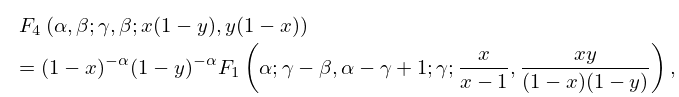
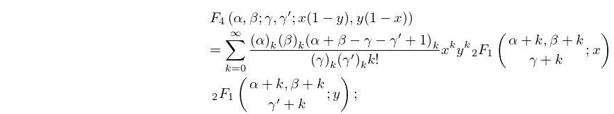
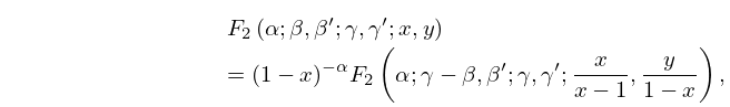
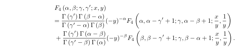
7: 16.16 Transformations of Variables
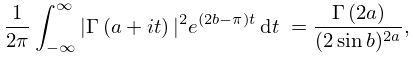
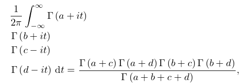
16.16.5 F 3 ( α , γ α ; β , γ β ; γ ; x , y ) = ( 1 y ) α + β γ F 1 2 ( α , β γ ; x + y x y ) ,
16.16.5_5 F 4 ( α , β ; γ , β ; x ( 1 y ) , y ( 1 x ) ) = ( 1 x ) α ( 1 y ) α F 1 ( α ; γ β , α γ + 1 ; γ ; x x 1 , x y ( 1 x ) ( 1 y ) ) ,
16.16.7 F 4 ( α , β ; γ , γ ; x ( 1 y ) , y ( 1 x ) ) = k = 0 ( α ) k ( β ) k ( α + β γ γ + 1 ) k ( γ ) k ( γ ) k k ! x k y k F 1 2 ( α + k , β + k γ + k ; x ) F 1 2 ( α + k , β + k γ + k ; y ) ;
16.16.9 F 2 ( α ; β , β ; γ , γ ; x , y ) = ( 1 x ) α F 2 ( α ; γ β , β ; γ , γ ; x x 1 , y 1 x ) ,
16.16.10 F 4 ( α , β ; γ , γ ; x , y ) = Γ ( γ ) Γ ( β α ) Γ ( γ α ) Γ ( β ) ( y ) α F 4 ( α , α γ + 1 ; γ , α β + 1 ; x y , 1 y ) + Γ ( γ ) Γ ( α β ) Γ ( γ β ) Γ ( α ) ( y ) β F 4 ( β , β γ + 1 ; γ , β α + 1 ; x y , 1 y ) .
8: 5.13 Integrals
5.13.1 1 2 π i c i c + i Γ ( s + a ) Γ ( b s ) z s d s = Γ ( a + b ) z a ( 1 + z ) a + b , ( a + b ) > 0 , a < c < b , | ph z | < π .
5.13.2 1 2 π | Γ ( a + i t ) | 2 e ( 2 b π ) t d t = Γ ( 2 a ) ( 2 sin b ) 2 a , a > 0 , 0 < b < π .
5.13.3 1 2 π Γ ( a + i t ) Γ ( b + i t ) Γ ( c i t ) Γ ( d i t ) d t = Γ ( a + c ) Γ ( a + d ) Γ ( b + c ) Γ ( b + d ) Γ ( a + b + c + d ) , a , b , c , d > 0 .
5.13.4 d t Γ ( a + t ) Γ ( b + t ) Γ ( c t ) Γ ( d t ) = Γ ( a + b + c + d 3 ) Γ ( a + c 1 ) Γ ( a + d 1 ) Γ ( b + c 1 ) Γ ( b + d 1 ) , ( a + b + c + d ) > 3 .
5.13.5 1 4 π k = 1 4 Γ ( a k + i t ) Γ ( a k i t ) Γ ( 2 i t ) Γ ( 2 i t ) d t = 1 j < k 4 Γ ( a j + a k ) Γ ( a 1 + a 2 + a 3 + a 4 ) , ( a k ) > 0 , k = 1 , 2 , 3 , 4 .
9: 5.22 Tables
Abramowitz and Stegun (1964, Chapter 6) tabulates Γ ( x ) , ln Γ ( x ) , ψ ( x ) , and ψ ( x ) for x = 1 ( .005 ) 2 to 10D; ψ ′′ ( x ) and ψ ( 3 ) ( x ) for x = 1 ( .01 ) 2 to 10D; Γ ( n ) , 1 / Γ ( n ) , Γ ( n + 1 2 ) , ψ ( n ) , log 10 Γ ( n ) , log 10 Γ ( n + 1 3 ) , log 10 Γ ( n + 1 2 ) , and log 10 Γ ( n + 2 3 ) for n = 1 ( 1 ) 101 to 8–11S; Γ ( n + 1 ) for n = 100 ( 100 ) 1000 to 20S. Zhang and Jin (1996, pp. 67–69 and 72) tabulates Γ ( x ) , 1 / Γ ( x ) , Γ ( x ) , ln Γ ( x ) , ψ ( x ) , ψ ( x ) , ψ ( x ) , and ψ ( x ) for x = 0 ( .1 ) 5 to 8D or 8S; Γ ( n + 1 ) for n = 0 ( 1 ) 100 ( 10 ) 250 ( 50 ) 500 ( 100 ) 3000 to 51S. … Abramov (1960) tabulates ln Γ ( x + i y ) for x = 1 ( .01 ) 2 , y = 0 ( .01 ) 4 to 6D. Abramowitz and Stegun (1964, Chapter 6) tabulates ln Γ ( x + i y ) for x = 1 ( .1 ) 2 , y = 0 ( .1 ) 10 to 12D. …Zhang and Jin (1996, pp. 70, 71, and 73) tabulates the real and imaginary parts of Γ ( x + i y ) , ln Γ ( x + i y ) , and ψ ( x + i y ) for x = 0.5 , 1 , 5 , 10 , y = 0 ( .5 ) 10 to 8S.
10: 30.6 Functions of Complex Argument
The solutions
𝑃𝑠 n m ( z , γ 2 ) ,
𝑄𝑠 n m ( z , γ 2 ) ,
of (30.2.1) with μ = m and λ = λ n m ( γ 2 ) are real when z ( 1 , ) , and their principal values (§4.2(i)) are obtained by analytic continuation to ( , 1 ] . … with A n ± m ( γ 2 ) as in (30.11.4). …