conjugate Poisson integral

SearchAdvancedHelp

(0.002 seconds)

11—20 of 462 matching pages

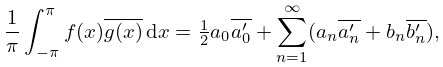
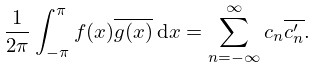
11: 1.8 Fourier Series

… ►

1.8.6_1 $$\frac{1}{\pi }{\int }_{-\pi }^{\pi }f(x)\overline{g(x)}dx=\frac{1}{2}{a}_0\overline{a_0^{\prime }}+\sum _{n=1}^{\mathrm{\infty }}(a_n\overline{a_n^{\prime }}+b_n\overline{b_n^{\prime }}),$$

ⓘ

Symbols:

$\pi$: the ratio of the circumference of a circle to its diameter, $\overline{z}$: complex conjugate, $dx$: differential of $x$ , $\int$: integral and $n$: nonnegative integer

Referenced by:

(1.8.13), (1.8.13), §1.8(i), §1.8(iv), Erratum (V1.2.0) Section 1.8

Permalink:

http://dlmf.nist.gov/1.8.E6_1

Encodings:

pMML, png, TeX

Rearrangement (effective with 1.2.0):

This equation, which was originally (1.8.13), was moved here.

See also:

Annotations for §1.8(i), §1.8(i), §1.8 and Ch.1

►

1.8.6_2 $$\frac{1}{2\pi }{\int }_{-\pi }^{\pi }f(x)\overline{g(x)}dx=\sum _{n=-\mathrm{\infty }}^{\mathrm{\infty }}{c}_n\overline{c_n^{\prime }}.$$

ⓘ

Symbols:

$\pi$: the ratio of the circumference of a circle to its diameter, $\overline{z}$: complex conjugate, $dx$: differential of $x$ , $\int$: integral and $n$: nonnegative integer

Referenced by:

§1.8(i), Erratum (V1.2.0) Section 1.8

Permalink:

http://dlmf.nist.gov/1.8.E6_2

Encodings:

pMML, png, TeX

Addition (effective with 1.2.0):

This equation was added.

See also:

Annotations for §1.8(i), §1.8(i), §1.8 and Ch.1

… ►(1.8.10) continues to apply if either $a$ or $b$ or both are infinite and/or $f(x)$ has finitely many singularities in $(a,b)$, provided that the integral converges uniformly (§1.5(iv)) at $a,b$, and the singularities for all sufficiently large $\lambda$. … ►

§1.8(iv) Poisson’s Summation Formula

… ►It follows from definition (1.14.1) that the integral in (1.8.14) is equal to $\sqrt{2\pi }ℱ\left(f\right)\left(-2\pi n\right)$. …

12: 18.33 Polynomials Orthogonal on the Unit Circle

… ►

18.33.1 $$\frac{1}{2\pi \mathrm{i}}{\int }_{|z|=1}{\varphi }_n(z)\overline{{\varphi }_m(z)}w(z)\frac{dz}{z}={\delta }_{n,m},$$

ⓘ

Symbols:

${\delta }_{j,k}$: Kronecker delta, $\pi$: the ratio of the circumference of a circle to its diameter, $\overline{z}$: complex conjugate, $dx$: differential of $x$ , $\mathrm{i}$: imaginary unit, $\int$: integral, $w(x)$: weight function, $z$: complex variable, $m$: nonnegative integer, $n$: nonnegative integer and ${\varphi }_n(z)$: polynomials

Referenced by:

§18.33(vi)

Permalink:

http://dlmf.nist.gov/18.33.E1

Encodings:

pMML, png, TeX

See also:

Annotations for §18.33(i), §18.33 and Ch.18

►where the bar signifies complex conjugate. … ►where the bar again signifies complex conjugate. … ►where the bar signifies complex conjugate and ${\kappa }_n>0$, ${\kappa }_0=1$. … ►for $n>0$, while ${\mathrm{\Phi }}_1(z)=z-\overline{{\alpha }_0}$. …

13: 1.9 Calculus of a Complex Variable

… ►

Complex Conjugate

►

1.9.11 $$\overline{z}=x-\mathrm{i}y,$$

ⓘ

Defines:

$\overline{z}$: complex conjugate

Symbols:

$\mathrm{i}$: imaginary unit and $z$: variable

A&S Ref:

3.7.7

Permalink:

http://dlmf.nist.gov/1.9.E11

Encodings:

pMML, png, TeX

See also:

Annotations for §1.9(i), §1.9(i), §1.9 and Ch.1

… ►If $f(z(t_0))=\mathrm{\infty }$, $a\le t_0\le b$, then the integral is defined analogously to the infinite integrals in §1.4(v). … ►

Cauchy’s Integral Formula

… ►

Poisson Integral

…

14: 36.8 Convergent Series Expansions

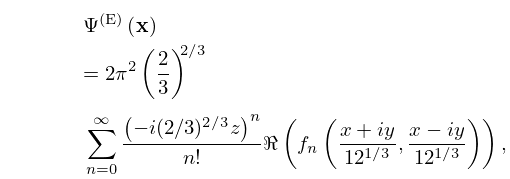
§36.8 Convergent Series Expansions

… ►For multinomial power series for ${\mathrm{\Psi }}_K\left(𝐱\right)$, see Connor and Curtis (1982). ►

36.8.3 $$\frac{3^{2/3}}{4{\pi }^2}{\mathrm{\Psi }}^{(\mathrm{H})}\left(3^{1/3}𝐱\right)=\mathrm{Ai}\left(x\right)\mathrm{Ai}\left(y\right)\sum _{n=0}^{\mathrm{\infty }}{(-3^{-1/3}\mathrm{i}z)}^n\frac{c_n(x)c_n(y)}{n!}+\mathrm{Ai}\left(x\right){\mathrm{Ai}}^{\prime }\left(y\right)\sum _{n=2}^{\mathrm{\infty }}{(-3^{-1/3}\mathrm{i}z)}^n\frac{c_n(x)d_n(y)}{n!}+{\mathrm{Ai}}^{\prime }\left(x\right)\mathrm{Ai}\left(y\right)\sum _{n=2}^{\mathrm{\infty }}{(-3^{-1/3}\mathrm{i}z)}^n\frac{d_n(x)c_n(y)}{n!}+{\mathrm{Ai}}^{\prime }\left(x\right){\mathrm{Ai}}^{\prime }\left(y\right)\sum _{n=1}^{\mathrm{\infty }}{(-3^{-1/3}\mathrm{i}z)}^n\frac{d_n(x)d_n(y)}{n!},$$

ⓘ

Symbols:

$\mathrm{Ai}\left(z\right)$: Airy function, $\pi$: the ratio of the circumference of a circle to its diameter, $!$: factorial (as in $n!$), ${\mathrm{\Psi }}^{(\mathrm{H})}\left(𝐱\right)$: hyperbolic umbilic canonical integral function, $\mathrm{i}$: imaginary unit, $y$: real parameter, $z$: real parameter, $m$: integer, $x$: real parameter, $c_n(t)$: coefficients and $d_n(t)$: coefficients

Referenced by:

§36.8

Permalink:

http://dlmf.nist.gov/36.8.E3

Encodings:

pMML, png, TeX

See also:

Annotations for §36.8 and Ch.36

… ►

36.8.4 $${\mathrm{\Psi }}^{(\mathrm{E})}\left(𝐱\right)=2{\pi }^2{\left(\frac{2}{3}\right)}^{2/3}\sum _{n=0}^{\mathrm{\infty }}\frac{{\left(-\mathrm{i}{(2/3)}^{2/3}z\right)}^n}{n!}\mathrm{\Re }\left(f_n(\frac{x+\mathrm{i}y}{{12}^{1/3}},\frac{x-\mathrm{i}y}{{12}^{1/3}})\right),$$

ⓘ

Symbols:

$\pi$: the ratio of the circumference of a circle to its diameter, ${\mathrm{\Psi }}^{(\mathrm{E})}\left(𝐱\right)$: elliptic umbilic canonical integral function, $!$: factorial (as in $n!$), $\mathrm{i}$: imaginary unit, $\mathrm{\Re }$: real part, $y$: real parameter, $z$: real parameter, $m$: integer, $x$: real parameter and $f_n$: function

Referenced by:

§36.8

Permalink:

http://dlmf.nist.gov/36.8.E4

Encodings:

pMML, png, TeX

See also:

Annotations for §36.8 and Ch.36

… ►

36.8.5 $$f_n(\zeta ,\overline{\zeta })=c_n(\zeta )c_n(\overline{\zeta })\mathrm{Ai}\left(\zeta \right)\mathrm{Bi}\left(\overline{\zeta }\right)+c_n(\zeta )d_n(\overline{\zeta })\mathrm{Ai}\left(\zeta \right){\mathrm{Bi}}^{\prime }\left(\overline{\zeta }\right)+d_n(\zeta )c_n(\overline{\zeta }){\mathrm{Ai}}^{\prime }\left(\zeta \right)\mathrm{Bi}\left(\overline{\zeta }\right)+d_n(\zeta )d_n(\overline{\zeta }){\mathrm{Ai}}^{\prime }\left(\zeta \right){\mathrm{Bi}}^{\prime }\left(\overline{\zeta }\right),$$

ⓘ

Defines:

$f_n$: function (locally)

Symbols:

$\mathrm{Ai}\left(z\right)$: Airy function, $\mathrm{Bi}\left(z\right)$: Airy function, $\overline{z}$: complex conjugate, $m$: integer, $c_n(t)$: coefficients and $d_n(t)$: coefficients

Permalink:

http://dlmf.nist.gov/36.8.E5

Encodings:

pMML, png, TeX

See also:

Annotations for §36.8 and Ch.36

…

15: Bibliography H

… ►

Une $q$-intégrale de Selberg et Askey. SIAM J. Math. Anal. 19 (6), pp. 1475–1489.

ⓘ

External Links:

ISSN 0036-1410, Document, MathReview (R. A. Askey), ZentralBlatt

Referenced by:

§17.13.

Encodings:

BibTeX

… ►

Certain integrals that contain a probability function. Bul. Akad. Štiince RSS Moldoven. 1975 (2), pp. 86–88, 95 (Russian).

ⓘ

External Links:

MathReview (C. Tanaka)

Referenced by:

§7.14(iii).

Encodings:

BibTeX

… ►

An Euler-Maclaurin-type formula involving conjugate Bernoulli polynomials and an application to $\zeta (2m+1)$ . Commun. Appl. Anal. 1 (1), pp. 15–32.

ⓘ

External Links:

ISSN 1083-2564, MathReview (Pavel Guerzhoy), ZentralBlatt

Referenced by:

§24.16(iii).

Encodings:

BibTeX

►

A Boole-type Formula involving Conjugate Euler Polynomials. In Charlemagne and his Heritage. 1200 Years of Civilization and Science in Europe, Vol. 2 (Aachen, 1995), P.L. Butzer, H. Th. Jongen, and W. Oberschelp (Eds.), pp. 361–375.

ⓘ

External Links:

ISBN 2-503-50674-7, MathReview (Bruce C. Berndt), ZentralBlatt

Referenced by:

§24.16(iii).

Encodings:

BibTeX

… ►

Solutions of Poisson’s equation in channel-like geometries. Comput. Phys. Comm. 115 (1), pp. 45–68.

ⓘ

External Links:

ISSN 0010-4655, Document, Code, MathReview Entry, ZentralBlatt

Referenced by:

§14.31(i).

Encodings:

BibTeX

…

16: 14.31 Other Applications

… ►

§14.31(i) Toroidal Functions

►Applications of toroidal functions include expansion of vacuum magnetic fields in stellarators and tokamaks (van Milligen and López Fraguas (1994)), analytic solutions of Poisson’s equation in channel-like geometries (Hoyles et al. (1998)), and Dirichlet problems with toroidal symmetry (Gil et al. (2000)). … ►These functions are also used in the Mehler–Fock integral transform (§14.20(vi)) for problems in potential and heat theory, and in elementary particle physics (Sneddon (1972, Chapter 7) and Braaksma and Meulenbeld (1967)). …

17: 1.18 Linear Second Order Differential Operators and Eigenfunction Expansions

… ►A complex linear vector space $V$ is called an inner product space if an inner product $⟨u,v⟩\in ℂ$ is defined for all $u,v\in V$ with the properties: (i) $⟨u,v⟩$ is complex linear in $u$; (ii) $⟨u,v⟩=\overline{⟨v,u⟩}$; (iii) $⟨v,v⟩\ge 0$; (iv) if $⟨v,v⟩=0$ then $v=0$. … ►where the integral kernel is given by … ►Should an eigenvalue correspond to more than a single linearly independent eigenfunction, namely a multiplicity greater than one, all such eigenfunctions will always be implied as being part of any sums or integrals over the spectrum. … ►Also, because $q$ is real-valued, $f\in N_z$ iff $\overline{f}\in N_{\overline{z}}$. … ►Integral transforms (10.22.78) and (10.22.79) are examples of the utility of these extensions. …

18: 7.13 Zeros

… ►The other zeros of $\mathrm{erf}z$ are $-z_n$, ${\overline{z}}_n$, $-{\overline{z}}_n$. … ►The other zeros of $\mathrm{erfc}z$ are ${\overline{z}}_n$. The zeros of $w\left(z\right)$ are $\mathrm{i}{z}_n$ and $\mathrm{i}{\overline{z}}_n$. … ►

§7.13(iii) Zeros of the Fresnel Integrals

… ►Then $-z_n$, ${\overline{z}}_n$, $-{\overline{z}}_n$, $\mathrm{i}{z}_n$, $-\mathrm{i}{z}_n$, $\mathrm{i}{\overline{z}}_n$, $-\mathrm{i}{\overline{z}}_n$ are also zeros of the same integral. …

19: 19.18 Derivatives and Differential Equations

… ►

§19.18(i) Derivatives

… ►

§19.18(ii) Differential Equations

… ►and also a system of $n(n-1)/2$ Euler–Poisson differential equations (of which only $n-1$ are independent): … ►The next four differential equations apply to the complete case of $R_F$ and $R_G$ in the form $R_{-a}(\frac{1}{2},\frac{1}{2};z_1,z_2)$ (see (19.16.20) and (19.16.23)). ►The function $w=R_{-a}(\frac{1}{2},\frac{1}{2};x+y,x-y)$ satisfies an Euler–Poisson–Darboux equation: …

20: 36.11 Leading-Order Asymptotics

§36.11 Leading-Order Asymptotics

… ►and far from the bifurcation set, the cuspoid canonical integrals are approximated by … ►

36.11.5 $${\mathrm{\Psi }}_3\left(0,y,0\right)=\overline{{\mathrm{\Psi }}_3(0,-y,0)}=\exp \left(\frac{1}{4}\mathrm{i}\pi \right)\sqrt{\pi /y}\left(1-(\mathrm{i}/\sqrt{3})\exp \left(\frac{3}{2}\mathrm{i}{(2y/5)}^{5/3}\right)+o\left(1\right)\right),$$ $y\to +\mathrm{\infty }$.

ⓘ

Symbols:

${\mathrm{\Psi }}_K\left(𝐱\right)$: canonical integral function, $\pi$: the ratio of the circumference of a circle to its diameter, $\overline{z}$: complex conjugate, $\exp z$: exponential function, $\mathrm{i}$: imaginary unit, $o\left(x\right)$: order less than and $y$: real parameter

Permalink:

http://dlmf.nist.gov/36.11.E5

Encodings:

pMML, png, TeX

See also:

Annotations for §36.11, §36.11 and Ch.36

… ►

36.11.7 $${\mathrm{\Psi }}^{(\mathrm{E})}\left(0,0,z\right)=\frac{\pi }{z}\left(\mathrm{i}+\sqrt{3}\exp \left(\frac{4}{27}\mathrm{i}{z}^3\right)+o\left(1\right)\right),$$ $z\to \pm \mathrm{\infty }$,

ⓘ

Symbols:

$\pi$: the ratio of the circumference of a circle to its diameter, ${\mathrm{\Psi }}^{(\mathrm{E})}\left(𝐱\right)$: elliptic umbilic canonical integral function, $\exp z$: exponential function, $\mathrm{i}$: imaginary unit, $o\left(x\right)$: order less than and $z$: real parameter

Permalink:

http://dlmf.nist.gov/36.11.E7

Encodings:

pMML, png, TeX

See also:

Annotations for §36.11, §36.11 and Ch.36

►

36.11.8 $${\mathrm{\Psi }}^{(\mathrm{H})}\left(0,0,z\right)=\frac{2\pi }{z}\left(1-\frac{\mathrm{i}}{\sqrt{3}}\exp \left(\frac{1}{27}\mathrm{i}{z}^3\right)+o\left(1\right)\right),$$ $z\to \pm \mathrm{\infty }$.

ⓘ

Symbols:

$\pi$: the ratio of the circumference of a circle to its diameter, $\exp z$: exponential function, ${\mathrm{\Psi }}^{(\mathrm{H})}\left(𝐱\right)$: hyperbolic umbilic canonical integral function, $\mathrm{i}$: imaginary unit, $o\left(x\right)$: order less than and $z$: real parameter

Permalink:

http://dlmf.nist.gov/36.11.E8

Encodings:

pMML, png, TeX

See also:

Annotations for §36.11, §36.11 and Ch.36