confluent form

SearchAdvancedHelp

(0.003 seconds)

11—20 of 41 matching pages

11: 13.27 Mathematical Applications

§13.27 Mathematical Applications

►Confluent hypergeometric functions are connected with representations of the group of third-order triangular matrices. The elements of this group are of the form … …

12: 13.14 Definitions and Basic Properties

… ►Although $M_{\kappa ,\mu }\left(z\right)$ does not exist when $2\mu =-1,-2,-3,\mathrm{\dots }$, many formulas containing $M_{\kappa ,\mu }\left(z\right)$ continue to apply in their limiting form. …

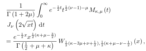
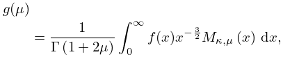
13: 13.4 Integral Representations

… ►

13.4.1 $$𝐌(a,b,z)=\frac{1}{\mathrm{\Gamma }\left(a\right)\mathrm{\Gamma }\left(b-a\right)}{\int }_0^1{\mathrm{e}}^{zt}{t}^{a-1}{(1-t)}^{b-a-1}dt,$$ $\mathrm{\Re }b>\mathrm{\Re }a>0$,

ⓘ

Symbols:

$\mathrm{\Gamma }\left(z\right)$: gamma function, $𝐌(a,b,z)$: Olver’s confluent hypergeometric function, $dx$: differential of $x$ , $\mathrm{e}$: base of natural logarithm, $\int$: integral, $\mathrm{\Re }$: real part and $z$: complex variable

A&S Ref:

13.2.1 (in different form)

Referenced by:

§13.10(v), §13.29(iii)

Permalink:

http://dlmf.nist.gov/13.4.E1

Encodings:

pMML, png, TeX

See also:

Annotations for §13.4(i), §13.4 and Ch.13

… ►

13.4.16 $$𝐌(a,b,-z)=\frac{1}{2\pi \mathrm{i}\mathrm{\Gamma }\left(a\right)}{\int }_{-\mathrm{i}\mathrm{\infty }}^{\mathrm{i}\mathrm{\infty }}\frac{\mathrm{\Gamma }\left(a+t\right)\mathrm{\Gamma }\left(-t\right)}{\mathrm{\Gamma }\left(b+t\right)}{z}^{t}dt,$$ ,

ⓘ

Symbols:

$\mathrm{\Gamma }\left(z\right)$: gamma function, $𝐌(a,b,z)$: Olver’s confluent hypergeometric function, $\pi$: the ratio of the circumference of a circle to its diameter, $dx$: differential of $x$ , $\mathrm{i}$: imaginary unit, $\int$: integral, $\mathrm{ph}$: phase and $z$: complex variable

Keywords:

Mellin transform

A&S Ref:

13.2.9 (in different form)

Permalink:

http://dlmf.nist.gov/13.4.E16

Encodings:

pMML, png, TeX

See also:

Annotations for §13.4(iii), §13.4 and Ch.13

…

14: 13.3 Recurrence Relations and Derivatives

… ►

13.3.14 $$(a+1)zU(a+2,b+2,z)+(z-b)U(a+1,b+1,z)-U(a,b,z)=0.$$

ⓘ

Symbols:

$U(a,b,z)$: Kummer confluent hypergeometric function and $z$: complex variable

Referenced by:

§13.3(i)

Permalink:

http://dlmf.nist.gov/13.3.E14

Encodings:

pMML, png, TeX

See also:

Annotations for §13.3(i), §13.3 and Ch.13

…

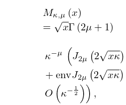
15: 13.8 Asymptotic Approximations for Large Parameters

… ►

13.8.9 $$M(a,b,x)=\mathrm{\Gamma }\left(b\right){\mathrm{e}}^{\frac{1}{2}x}{\left((\frac{1}{2}b-a)x\right)}^{\frac{1}{2}-\frac{1}{2}b}\left(J_{b-1}\left(\sqrt{2x(b-2a)}\right)+\mathrm{env}{J}_{b-1}\left(\sqrt{2x(b-2a)}\right)O\left({\left|a\right|}^{-\frac{1}{2}}\right)\right),$$

ⓘ

Symbols:

$J_{\nu }\left(z\right)$: Bessel function of the first kind, $O\left(x\right)$: order not exceeding, $\mathrm{\Gamma }\left(z\right)$: gamma function, $M(a,b,z)$: $={}_1{}^{}F_1^{}(a;b;z)$ Kummer confluent hypergeometric function, $\mathrm{env}{J}_{\nu }\left(x\right)$: envelope of Bessel function $J_{\nu }\left(x\right)$ , $\mathrm{e}$: base of natural logarithm and $x$: real variable

A&S Ref:

13.5.13 (in different form)

Referenced by:

§13.9(i)

Permalink:

http://dlmf.nist.gov/13.8.E9

Encodings:

pMML, png, TeX

See also:

Annotations for §13.8(iii), §13.8 and Ch.13

… ►

13.8.10 $$U(a,b,x)=\mathrm{\Gamma }\left(\frac{1}{2}b-a+\frac{1}{2}\right){\mathrm{e}}^{\frac{1}{2}x}{x}^{\frac{1}{2}-\frac{1}{2}b}\left(\cos \left(a\pi \right)J_{b-1}\left(\sqrt{2x(b-2a)}\right)-\sin \left(a\pi \right)Y_{b-1}\left(\sqrt{2x(b-2a)}\right)+\mathrm{env}{Y}_{b-1}\left(\sqrt{2x(b-2a)}\right)O\left({\left|a\right|}^{-\frac{1}{2}}\right)\right),$$

ⓘ

Symbols:

$J_{\nu }\left(z\right)$: Bessel function of the first kind, $Y_{\nu }\left(z\right)$: Bessel function of the second kind, $O\left(x\right)$: order not exceeding, $\mathrm{\Gamma }\left(z\right)$: gamma function, $U(a,b,z)$: Kummer confluent hypergeometric function, $\pi$: the ratio of the circumference of a circle to its diameter, $\cos z$: cosine function, $\mathrm{env}{Y}_{\nu }\left(x\right)$: envelope of Bessel function $Y_{\nu }\left(x\right)$ , $\mathrm{e}$: base of natural logarithm, $\sin z$: sine function and $x$: real variable

A&S Ref:

13.5.15 (in different form)

Referenced by:

§13.9(ii)

Permalink:

http://dlmf.nist.gov/13.8.E10

Encodings:

pMML, png, TeX

See also:

Annotations for §13.8(iii), §13.8 and Ch.13

…

16: 13.21 Uniform Asymptotic Approximations for Large $\kappa$

… ►

13.21.1 $$M_{\kappa ,\mu }\left(x\right)=\sqrt{x}\mathrm{\Gamma }\left(2\mu +1\right){\kappa }^{-\mu }\left(J_{2\mu }\left(2\sqrt{x\kappa }\right)+\mathrm{env}{J}_{2\mu }\left(2\sqrt{x\kappa }\right)O\left({\kappa }^{-\frac{1}{2}}\right)\right),$$

ⓘ

Symbols:

$J_{\nu }\left(z\right)$: Bessel function of the first kind, $O\left(x\right)$: order not exceeding, $\mathrm{\Gamma }\left(z\right)$: gamma function, $M_{\kappa ,\mu }\left(z\right)$: Whittaker confluent hypergeometric function, $\mathrm{env}{J}_{\nu }\left(x\right)$: envelope of Bessel function $J_{\nu }\left(x\right)$ and $x$: real variable

Permalink:

http://dlmf.nist.gov/13.21.E1

Encodings:

pMML, png, TeX

See also:

Annotations for §13.21(i), §13.21 and Ch.13

… ►

13.21.6 $$M_{-\kappa ,\mu }\left(4\kappa x\right)=\frac{2\mathrm{\Gamma }\left(2\mu +1\right)}{{\kappa }^{\mu -\frac{1}{2}}}{\left(\frac{x\zeta }{1+x}\right)}^{\frac{1}{4}}{I}_{2\mu }\left(4\kappa {\zeta }^{\frac{1}{2}}\right)\left(1+O\left({\kappa }^{-1}\right)\right),$$

ⓘ

Symbols:

$O\left(x\right)$: order not exceeding, $\mathrm{\Gamma }\left(z\right)$: gamma function, $M_{\kappa ,\mu }\left(z\right)$: Whittaker confluent hypergeometric function, $I_{\nu }\left(z\right)$: modified Bessel function of the first kind and $x$: real variable

Referenced by:

§13.21(i)

Permalink:

http://dlmf.nist.gov/13.21.E6

Encodings:

pMML, png, TeX

See also:

Annotations for §13.21(i), §13.21 and Ch.13

►

13.21.7 $$W_{-\kappa ,\mu }\left(4\kappa x\right)=\frac{\sqrt{8/\pi }{\mathrm{e}}^{\kappa }}{{\kappa }^{\kappa -\frac{1}{2}}}{\left(\frac{x\zeta }{1+x}\right)}^{\frac{1}{4}}{K}_{2\mu }\left(4\kappa {\zeta }^{\frac{1}{2}}\right)\left(1+O\left({\kappa }^{-1}\right)\right),$$

ⓘ

Symbols:

$O\left(x\right)$: order not exceeding, $W_{\kappa ,\mu }\left(z\right)$: Whittaker confluent hypergeometric function, $\pi$: the ratio of the circumference of a circle to its diameter, $\mathrm{e}$: base of natural logarithm, $K_{\nu }\left(z\right)$: modified Bessel function of the second kind and $x$: real variable

Referenced by:

§13.21(i)

Permalink:

http://dlmf.nist.gov/13.21.E7

Encodings:

pMML, png, TeX

See also:

Annotations for §13.21(i), §13.21 and Ch.13

… ►For a uniform asymptotic expansion in terms of Airy functions for $W_{\kappa ,\mu }\left(4\kappa x\right)$ when $\kappa$ is large and positive, $\mu$ is real with $|\mu |$ bounded, and $x\in [\delta ,\mathrm{\infty })$ see Olver (1997b, Chapter 11, Ex. 7.3). This expansion is simpler in form than the expansions of Dunster (1989) that correspond to the approximations given in §13.21(iii), but the conditions on $\mu$ are more restrictive. …

17: Bibliography T

… ►

Uniform asymptotic expansions of confluent hypergeometric functions. J. Inst. Math. Appl. 22 (2), pp. 215–223.

ⓘ

External Links:

ISSN 0020-2932, Document, MathReview (F. W. J. Olver), ZentralBlatt

Referenced by:

§13.8(ii), §13.8(ii).

Encodings:

BibTeX

… ►

The numerical computation of the confluent hypergeometric function $U(a,b,z)$ . Numer. Math. 41 (1), pp. 63–82.

ⓘ

Notes:

Algol 60 variable-precision procedures are included.

External Links:

ISSN 0029-599X, Document, MathReview (H. E. Fettis), ZentralBlatt

Referenced by:

§13.29(iv), §13.32(ii).

Encodings:

BibTeX

►

Laplace type integrals: Transformation to standard form and uniform asymptotic expansions. Quart. Appl. Math. 43 (1), pp. 103–123.

ⓘ

External Links:

ISSN 0033-569X, FullText, MathReview (I. Fenyő), ZentralBlatt

Referenced by:

§2.4(i).

Encodings:

BibTeX

… ►

Uniform asymptotic expansions of a class of integrals in terms of modified Bessel functions, with application to confluent hypergeometric functions. SIAM J. Math. Anal. 21 (1), pp. 241–261.

ⓘ

External Links:

ISSN 0036-1410, Document, MathReview (Pablo Martín), ZentralBlatt

Referenced by:

§13.8(iii), §13.8(iii).

Encodings:

BibTeX

… ►

Algebraic transformations of hypergeometric functions and automorphic forms on Shimura curves. Trans. Amer. Math. Soc. 365 (12), pp. 6697–6729.

ⓘ

External Links:

ISSN 0002-9947, Document, FullText, MathReview (John M. Voight), ZentralBlatt

Referenced by:

§15.8(v), §15.8(v).

Encodings:

BibTeX

…

18: Mathematical Introduction

… ►Similarly in the case of confluent hypergeometric functions (§13.2(i)). ►Other examples are: (a) the notation for the Ferrers functions—also known as associated Legendre functions on the cut—for which existing notations can easily be confused with those for other associated Legendre functions (§14.1); (b) the spherical Bessel functions for which existing notations are unsymmetric and inelegant (§§10.47(i) and 10.47(ii)); and (c) elliptic integrals for which both Legendre’s forms and the more recent symmetric forms are treated fully (Chapter 19). … ►For equations or other technical information that appeared previously in AMS 55, the DLMF usually includes the corresponding AMS 55 equation number, or other form of reference, together with corrections, if needed. …

19: 18.11 Relations to Other Functions

… ►

Laguerre

… ►

Hermite

… ►

§18.11(ii) Formulas of Mehler–Heine Type

►

Jacobi

… ►

Hermite

…

20: 13.23 Integrals

… ►

13.23.8 $$\frac{1}{\mathrm{\Gamma }\left(1+2\mu \right)}{\int }_0^{\mathrm{\infty }}\cos \left(2xt\right){\mathrm{e}}^{-\frac{1}{2}{t}^2}{t}^{-2\mu -1}{M}_{\kappa ,\mu }\left(t^2\right)dt=\frac{\sqrt{\pi }{\mathrm{e}}^{-\frac{1}{2}{x}^2}{x}^{\mu +\kappa -1}}{2\mathrm{\Gamma }\left(\frac{1}{2}+\mu +\kappa \right)}{W}_{\frac{1}{2}\kappa -\frac{3}{2}\mu ,\frac{1}{2}\kappa +\frac{1}{2}\mu }\left(x^2\right),$$ $\mathrm{\Re }\left(\kappa +\mu \right)>-\frac{1}{2}$.

ⓘ

Symbols:

$\mathrm{\Gamma }\left(z\right)$: gamma function, $M_{\kappa ,\mu }\left(z\right)$: Whittaker confluent hypergeometric function, $W_{\kappa ,\mu }\left(z\right)$: Whittaker confluent hypergeometric function, $\pi$: the ratio of the circumference of a circle to its diameter, $\cos z$: cosine function, $dx$: differential of $x$ , $\mathrm{e}$: base of natural logarithm, $\int$: integral, $\mathrm{\Re }$: real part and $x$: real variable

Permalink:

http://dlmf.nist.gov/13.23.E8

Encodings:

pMML, png, TeX

See also:

Annotations for §13.23(ii), §13.23 and Ch.13

… ►

13.23.10 $$\frac{1}{\mathrm{\Gamma }\left(1+2\mu \right)}{\int }_0^{\mathrm{\infty }}{\mathrm{e}}^{-\frac{1}{2}t}{t}^{\frac{1}{2}(\nu -1)-\mu }{M}_{\kappa ,\mu }\left(t\right)J_{\nu }\left(2\sqrt{xt}\right)dt=\frac{{\mathrm{e}}^{-\frac{1}{2}x}{x}^{\frac{1}{2}(\kappa +\mu -\frac{3}{2})}}{\mathrm{\Gamma }\left(\frac{1}{2}+\mu +\kappa \right)}{W}_{\frac{1}{2}(\kappa -3\mu +\nu +\frac{1}{2}),\frac{1}{2}(\kappa +\mu -\nu -\frac{1}{2})}\left(x\right),$$ $x>0$, .

ⓘ

Symbols:

$J_{\nu }\left(z\right)$: Bessel function of the first kind, $\mathrm{\Gamma }\left(z\right)$: gamma function, $M_{\kappa ,\mu }\left(z\right)$: Whittaker confluent hypergeometric function, $W_{\kappa ,\mu }\left(z\right)$: Whittaker confluent hypergeometric function, $dx$: differential of $x$ , $\mathrm{e}$: base of natural logarithm, $\int$: integral, $\mathrm{\Re }$: real part and $x$: real variable

Permalink:

http://dlmf.nist.gov/13.23.E10

Encodings:

pMML, png, TeX

See also:

Annotations for §13.23(iii), §13.23 and Ch.13

… ►

13.23.13 $$g(\mu )=\frac{1}{\mathrm{\Gamma }\left(1+2\mu \right)}{\int }_0^{\mathrm{\infty }}f(x)x^{-\frac{3}{2}}{M}_{\kappa ,\mu }\left(x\right)dx,$$

ⓘ

Symbols:

$\mathrm{\Gamma }\left(z\right)$: gamma function, $M_{\kappa ,\mu }\left(z\right)$: Whittaker confluent hypergeometric function, $dx$: differential of $x$ , $\int$: integral and $x$: real variable

Permalink:

http://dlmf.nist.gov/13.23.E13

Encodings:

pMML, png, TeX

See also:

Annotations for §13.23(iv), §13.23 and Ch.13

►

13.23.14 $$f(x)=\frac{1}{\pi \mathrm{i}\sqrt{x}}{\int }_{{\mu }_1-\mathrm{i}\mathrm{\infty }}^{{\mu }_1+\mathrm{i}\mathrm{\infty }}\mu g(\mu )\mathrm{\Gamma }\left(\frac{1}{2}+\mu -\kappa \right)W_{\kappa ,\mu }\left(x\right)d\mu .$$

ⓘ

Symbols:

$\mathrm{\Gamma }\left(z\right)$: gamma function, $W_{\kappa ,\mu }\left(z\right)$: Whittaker confluent hypergeometric function, $\pi$: the ratio of the circumference of a circle to its diameter, $dx$: differential of $x$ , $\mathrm{i}$: imaginary unit, $\int$: integral and $x$: real variable

Permalink:

http://dlmf.nist.gov/13.23.E14

Encodings:

pMML, png, TeX

See also:

Annotations for §13.23(iv), §13.23 and Ch.13

… ►Additional integrals involving confluent hypergeometric functions can be found in Apelblat (1983, pp. 388–392), Erdélyi et al. (1954b), Gradshteyn and Ryzhik (2000, §7.6), and Prudnikov et al. (1990, §§1.13, 1.14, 2.19, 4.2.2). …