computation%20of%20coefficients

SearchAdvancedHelp

(0.003 seconds)

1—10 of 27 matching pages

1: Bibliography B

… ►

A program for computing the Riemann zeta function for complex argument. Comput. Phys. Comm. 20 (3), pp. 441–445.

ⓘ

Notes:

Double-precision Fortran, maximum accuracy 10S.

External Links:

Document, Code, ZentralBlatt

Referenced by:

1st item.

Encodings:

BibTeX

►

NJGRAF: An efficient program for calculation of general recoupling coefficients by graphical analysis, compatible with NJSYM. Comput. Phys. Comm. 50 (3), pp. 375–393.

ⓘ

External Links:

Document, Code

Referenced by:

1st item.

Encodings:

BibTeX

… ►

Coulomb functions (negative energies). Comput. Phys. Comm. 20 (3), pp. 447–458.

ⓘ

Notes:

Double-precision Fortran code.

External Links:

Document, Code

Referenced by:

1st item, 4th item.

Encodings:

BibTeX

… ►

Asymptotic Expansions for the Coefficient Functions Associated with Linear Second-order Differential Equations: The Simple Pole Case. In Asymptotic and Computational Analysis (Winnipeg, MB, 1989), R. Wong (Ed.), Lecture Notes in Pure and Applied Mathematics, Vol. 124, pp. 53–73.

ⓘ

External Links:

MathReview (John S. Lew), ZentralBlatt

Referenced by:

§2.8(iv).

Encodings:

BibTeX

… ►

A program to calculate a general recoupling coefficient. Comput. Phys. Comm. 1 (4), pp. 241–250.

ⓘ

Notes:

Single-precision Fortran

External Links:

Document, Code

Referenced by:

3rd item.

Encodings:

BibTeX

…

2: 11.6 Asymptotic Expansions

… ►

$c_3(\lambda )=20{\lambda }^{-6}-4{\lambda }^{-4},$

… ►These and higher coefficients $c_k(\lambda )$ can be computed via the representations in Nemes (2015b). …

3: 10.75 Tables

… ►

Olver (1962) provides tables for the uniform asymptotic expansions given in §10.20(i), including $\zeta$ and ${(4\zeta /(1-x^2))}^{\frac{1}{4}}$ as functions of $x$ $(=z)$ and the coefficients $A_k(\zeta )$, $B_k(\zeta )$, $C_k(\zeta )$, $D_k(\zeta )$ as functions of $\zeta$. These enable $J_{\nu }\left(\nu x\right)$, $Y_{\nu }\left(\nu x\right)$, $J_{\nu }^{\prime }\left(\nu x\right)$, $Y_{\nu }^{\prime }\left(\nu x\right)$ to be computed to 10S when $\nu \ge 15$, except in the neighborhoods of zeros.

… ►

Olver (1960) tabulates $j_{n,m}$, $J_n^{\prime }\left(j_{n,m}\right)$, $j_{n,m}^{\prime }$, $J_n\left(j_{n,m}^{\prime }\right)$, $y_{n,m}$, $Y_n^{\prime }\left(y_{n,m}\right)$, $y_{n,m}^{\prime }$, $Y_n\left(y_{n,m}^{\prime }\right)$, $n=0(\frac{1}{2})20⁤\frac{1}{2}$, $m=1(1)50$, 8D. Also included are tables of the coefficients in the uniform asymptotic expansions of these zeros and associated values as $n\to \mathrm{\infty }$; see §10.21(viii), and more fully Olver (1954).

… ►

Bickley et al. (1952) tabulates $x^{-n}{I}_n\left(x\right)$ or ${\mathrm{e}}^{-x}{I}_n\left(x\right)$, $x^n{K}_n\left(x\right)$ or ${\mathrm{e}}^x{K}_n\left(x\right)$, $n=2(1)20$, $x=0$(.01 or .1) 10(.1) 20, 8S; $I_n\left(x\right)$, $K_n\left(x\right)$, $n=0(1)20$, $x=0$ or $0.1(.1)20$, 10S.

►

Olver (1962) provides tables for the uniform asymptotic expansions given in §10.41(ii), including $\eta$ and the coefficients $U_k(p)$, $V_k(p)$ as functions of $p={(1+x^2)}^{-\frac{1}{2}}$. These enable $I_{\nu }\left(\nu x\right)$, $K_{\nu }\left(\nu x\right)$, $I_{\nu }^{\prime }\left(\nu x\right)$, $K_{\nu }^{\prime }\left(\nu x\right)$ to be computed to 10S when $\nu \ge 16$.

… ►

Olver (1960) tabulates $a_{n,m}^{\prime }$, ${𝗃}_n\left(a_{n,m}^{\prime }\right)$, $b_{n,m}^{\prime }$, ${𝗒}_n\left(b_{n,m}^{\prime }\right)$, $n=1(1)20$, $m=1(1)50$, 8D. Also included are tables of the coefficients in the uniform asymptotic expansions of these zeros and associated values as $n\to \mathrm{\infty }$.

…

4: Bibliography N

… ►

Tables of Lagrangian Interpolation Coefficients. Columbia University Press, New York.

ⓘ

Notes:

Technical Director: Arnold N. Lowan

External Links:

MathReview (W. Feller), ZentralBlatt

Referenced by:

§3.3(ii).

Encodings:

BibTeX

►

Modern Computing Methods. 2nd edition, Notes on Applied Science, No. 16, Her Majesty’s Stationery Office, London.

ⓘ

External Links:

MathReview (A. S. Householder), ZentralBlatt

Referenced by:

§3.8(iv).

Encodings:

BibTeX

… ►

On an integral transform involving a class of Mathieu functions. SIAM J. Math. Anal. 20 (6), pp. 1500–1513.

ⓘ

External Links:

ISSN 0036-1410, Document, MathReview (K. C. Gupta), ZentralBlatt

Referenced by:

§28.26(ii).

Encodings:

BibTeX

… ►

Reduction and evaluation of elliptic integrals. Math. Comp. 20 (94), pp. 223–231.

ⓘ

External Links:

FullText, MathReview (I. A. Stegun), ZentralBlatt

Referenced by:

§19.37(iv).

Encodings:

BibTeX

… ►

A table of integrals of the error functions. J. Res. Nat. Bur. Standards Sect B. 73B, pp. 1–20.

ⓘ

Notes:

See for additions and corrections same journal, Sect. B 75, 149–163 (1975)

External Links:

MathReview, ZentralBlatt

Referenced by:

§7.14(iii), §7.21, §7.7(iii).

Encodings:

BibTeX

…

5: Bibliography S

… ►

Recursive evaluation of $3j$- and $6j$- coefficients. Comput. Phys. Comm. 11 (2), pp. 269–278.

ⓘ

Notes:

Double-precision Fortran provided in 3 parts, $j_1$-recursion for $3j$-coefficients, $m_2$-recursion for $3j$-coefficients, and $j_1$-recursion for $6j$-coefficients

External Links:

Document, Code 1, Code 2, Code 3

Referenced by:

8th item.

Encodings:

BibTeX

… ►

New Fortran programs for angular momentum coefficients. Comput. Phys. Comm. 15 (3-4), pp. 227–235.

ⓘ

External Links:

Document

Referenced by:

§34.13.

Encodings:

BibTeX

►

Computation of angular momentum coefficients using sets of generalized hypergeometric functions. Comput. Phys. Comm. 22 (2-3), pp. 297–302.

ⓘ

External Links:

Document

Referenced by:

§34.13.

Encodings:

BibTeX

… ►

A Maple package for symmetric functions. J. Symbolic Comput. 20 (5-6), pp. 755–768.

ⓘ

Notes:

For software see John Stembridge’s home page. The SF package contains Maple software for zonal, Jack, and Macdonald polynomials.

External Links:

Home Page, ISSN 0747-7171, Document, MathReview, ZentralBlatt

Referenced by:

3rd item.

Encodings:

BibTeX

… ►

Numerical Methods Based on Sinc and Analytic Functions. Springer Series in Computational Mathematics, Vol. 20, Springer-Verlag, New York.

ⓘ

Notes:

Sinc-Pack, a set of 480 Matlab programs with a 470-page tutorial, is available for purchase from SINC, LLC by contacting Frank Stenger.

External Links:

ISBN 0-387-94008-1, MathReview (B. Boyanov), ZentralBlatt

Referenced by:

§3.3(vi), §3.4(i), §3.5(i).

Encodings:

BibTeX

…

6: Bibliography D

… ►

Computational properties of three-term recurrence relations for Kummer functions. J. Comput. Appl. Math. 233 (6), pp. 1505–1510.

ⓘ

External Links:

ISSN 0377-0427, Document, FullText, MathReview (Richard B. Paris), ZentralBlatt

Referenced by:

§13.29(iv), §13.29(iv).

Encodings:

BibTeX

… ►

Vector coupling coefficients as products of prime factors. Comput. Phys. Comm. 4 (2), pp. 268–274.

ⓘ

Notes:

Single-precision Fortran

External Links:

Document, Code

Referenced by:

4th item.

Encodings:

BibTeX

… ►

Complex zeros of cylinder functions. Math. Comp. 20 (94), pp. 215–222.

ⓘ

Notes:

For a numerical error in one of the zeros see Amos (1985).

External Links:

ISSN 0025-5718, FullText, MathReview, ZentralBlatt

Referenced by:

2nd item.

Encodings:

BibTeX

… ►

A program to calculate internal conversion coefficients for all atomic shells without screening. Comput. Phys. Comm. 2 (7), pp. 427–432.

ⓘ

Notes:

Single-precision Fortran

External Links:

Document, Code

Referenced by:

1st item.

Encodings:

BibTeX

… ►

Uniform asymptotic expansions for Whittaker’s confluent hypergeometric functions. SIAM J. Math. Anal. 20 (3), pp. 744–760.

ⓘ

Notes:

(This reference has several typographical errors.)

External Links:

ISSN 0036-1410, Document, MathReview (F. W. J. Olver), ZentralBlatt

Referenced by:

§13.21(ii), §13.21(iii), §13.21(iv).

Encodings:

BibTeX

…

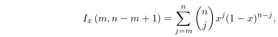
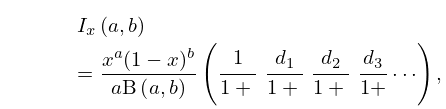
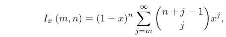
7: 8.17 Incomplete Beta Functions

… ►

8.17.5 $$I_x(m,n-m+1)=\sum _{j=m}^n\left(\genfrac{}{}{0.0pt}{}{n}{j}\right)x^j{(1-x)}^{n-j},$$ $m,n$ positive integers; .

ⓘ

Symbols:

$I_x(a,b)$: incomplete beta function, $\left(\genfrac{}{}{0.0pt}{}{m}{n}\right)$: binomial coefficient, $n$: nonnegative integer and $x$: variable

A&S Ref:

6.6.4 (Relation to the Binomial Expansion)

Referenced by:

§8.17(i), §8.17(vii), Erratum (V1.0.5) for Subsection 8.17(i)

Permalink:

http://dlmf.nist.gov/8.17.E5

Encodings:

pMML, png, TeX

See also:

Annotations for §8.17(i), §8.17 and Ch.8

… ►

8.17.22 $$I_x(a,b)=\frac{x^a{(1-x)}^b}{a\mathrm{B}(a,b)}\left(\frac{1}{1+}\frac{d_1}{1+}\frac{d_2}{1+}\frac{d_3}{1+}\mathrm{\cdots }\right),$$

ⓘ

Symbols:

$\mathrm{B}(a,b)$: beta function, $I_x(a,b)$: incomplete beta function, $a$: parameter, $d_m$: coefficients, $b$: parameter and $x$: variable

Referenced by:

§8.17(v)

Permalink:

http://dlmf.nist.gov/8.17.E22

Encodings:

pMML, png, TeX

See also:

Annotations for §8.17(v), §8.17 and Ch.8

►where … ►For $x>(a+1)/(a+b+2)$ or , more rapid convergence is obtained by computing $I_{1-x}(b,a)$ and using (8.17.4). … ►

8.17.24 $$I_x(m,n)={(1-x)}^n\sum _{j=m}^{\mathrm{\infty }}\left(\genfrac{}{}{0.0pt}{}{n+j-1}{j}\right)x^j,$$ $m,n$ positive integers; .

ⓘ

Symbols:

$I_x(a,b)$: incomplete beta function, $\left(\genfrac{}{}{0.0pt}{}{m}{n}\right)$: binomial coefficient, $n$: nonnegative integer and $x$: variable

A&S Ref:

26.5.26 (The upper limit of summation has been corrected.)

Referenced by:

§8.17(i), Erratum (V1.0.5) for Chapters 8, 20, 36

Permalink:

http://dlmf.nist.gov/8.17.E24

Encodings:

pMML, png, TeX

Addition (effective with 1.0.5):

This equation is the same as Equation (26.5.26) of Abramowitz and Stegun (1964), except that the upper limit of the summation has been corrected to $\mathrm{\infty }$.

Suggested 2011-03-23 by Stephen Bourn

See also:

Annotations for §8.17(vii), §8.17 and Ch.8

…

8: 3.8 Nonlinear Equations

… ►

§3.8(iv) Zeros of Polynomials

… ►However, when the coefficients are all real, complex arithmetic can be avoided by the following iterative process. … ►For further information on the computation of zeros of polynomials see McNamee (2007). … ►Consider $x=20$ and $j=19$. We have $p^{\prime }(20)=19!$ and $a_{19}=1+2+\mathrm{\cdots }+20=210$. …

9: 6.20 Approximations

… ►

Cody and Thacher (1968) provides minimax rational approximations for $E_1\left(x\right)$, with accuracies up to 20S.

►

Cody and Thacher (1969) provides minimax rational approximations for $\mathrm{Ei}\left(x\right)$, with accuracies up to 20S.

►

MacLeod (1996b) provides rational approximations for the sine and cosine integrals and for the auxiliary functions $\mathrm{f}$ and $\mathrm{g}$, with accuracies up to 20S.

… ►

Luke (1969b, pp. 321–322) covers $\mathrm{Ein}\left(x\right)$ and $-\mathrm{Ein}\left(-x\right)$ for $0\le x\le 8$ (the Chebyshev coefficients are given to 20D); $E_1\left(x\right)$ for $x\ge 5$ (20D), and $\mathrm{Ei}\left(x\right)$ for $x\ge 8$ (15D). Coefficients for the sine and cosine integrals are given on pp. 325–327.

►

Luke (1969b, p. 25) gives a Chebyshev expansion near infinity for the confluent hypergeometric $U$-function (§13.2(i)) from which Chebyshev expansions near infinity for $E_1\left(z\right)$, $\mathrm{f}\left(z\right)$, and $\mathrm{g}\left(z\right)$ follow by using (6.11.2) and (6.11.3). Luke also includes a recursion scheme for computing the coefficients in the expansions of the $U$ functions. If the scheme can be used in backward direction.

…

10: Bibliography M

… ►

Computation of inhomogeneous Airy functions. J. Comput. Appl. Math. 53 (1), pp. 109–116.

ⓘ

External Links:

ISSN 0377-0427, Document, MathReview (Dumitru Acu), ZentralBlatt

Referenced by:

1st item.

Encodings:

BibTeX

… ►

The efficient computation of some generalised exponential integrals. J. Comput. Appl. Math. 148 (2), pp. 363–374.

ⓘ

External Links:

ISSN 0377-0427, Document, MathReview, ZentralBlatt

Referenced by:

§8.19(v).

Encodings:

BibTeX

… ►

Painlevé-type differential equations for the recurrence coefficients of semi-classical orthogonal polynomials. J. Comput. Appl. Math. 57 (1-2), pp. 215–237.

ⓘ

External Links:

ISSN 0377-0427, Document, MathReview (Leonid B. Golinskiĭ), ZentralBlatt

Referenced by:

§32.15.

Encodings:

BibTeX

… ►

The computation of elementary functions in radix $2^p$ . Computing 53 (3-4), pp. 219–232.

ⓘ

Notes:

International Symposium on Scientific Computing, Computer Arithmetic and Validated Numerics (Vienna, 1993)

External Links:

ISSN 0010-485X, Document, MathReview, ZentralBlatt

Referenced by:

§4.45(i).

Encodings:

BibTeX

… ►

The $q$-analogue of the Laguerre polynomials. J. Math. Anal. Appl. 81 (1), pp. 20–47.

ⓘ

External Links:

ISSN 0022-247X, Document, MathReview (R. A. Askey), ZentralBlatt

Referenced by:

§18.27(v).

Encodings:

BibTeX

…