complex%20variables

SearchAdvancedHelp

(0.004 seconds)

1—10 of 34 matching pages

1: 6.19 Tables

… ►

§6.19(ii) Real Variables

… ►

Zhang and Jin (1996, pp. 652, 689) includes $\mathrm{Si}\left(x\right)$, $\mathrm{Ci}\left(x\right)$, $x=0(.5)20(2)30$, 8D; $\mathrm{Ei}\left(x\right)$, $E_1\left(x\right)$, $x=[0,100]$, 8S.

►

§6.19(iii) Complex Variables, $z=x+\mathrm{i}y$

►

Abramowitz and Stegun (1964, Chapter 5) includes the real and imaginary parts of $z{\mathrm{e}}^z{E}_1\left(z\right)$, $x=-19(1)20$, $y=0(1)20$, 6D; ${\mathrm{e}}^z{E}_1\left(z\right)$, $x=-4(.5)-2$, $y=0(.2)1$, 6D; $E_1\left(z\right)+\ln z$, $x=-2(.5)2.5$, $y=0(.2)1$, 6D.

►

Zhang and Jin (1996, pp. 690–692) includes the real and imaginary parts of $E_1\left(z\right)$, $\pm x=0.5,1,3,5,10,15,20,50,100$, $y=0(.5)1(1)5(5)30,50,100$, 8S.

2: Bibliography B

… ►

Pionic atoms. Annual Review of Nuclear and Particle Science 20, pp. 467–508.

ⓘ

External Links:

Document

Referenced by:

§33.22(iv).

Encodings:

BibTeX

… ►

A program for computing the Riemann zeta function for complex argument. Comput. Phys. Comm. 20 (3), pp. 441–445.

ⓘ

Notes:

Double-precision Fortran, maximum accuracy 10S.

External Links:

Document, Code, ZentralBlatt

Referenced by:

1st item.

Encodings:

BibTeX

… ►

Coulomb functions (negative energies). Comput. Phys. Comm. 20 (3), pp. 447–458.

ⓘ

Notes:

Double-precision Fortran code.

External Links:

Document, Code

Referenced by:

1st item, 4th item.

Encodings:

BibTeX

… ►

Some solutions of the problem of forced convection. Philos. Mag. Series 7 20, pp. 322–343.

ⓘ

External Links:

Document, ZentralBlatt

Referenced by:

§10.73(iv).

Encodings:

BibTeX

… ►

Several Complex Variables. Princeton Mathematical Series, Vol. 10, Princeton University Press, Princeton, N.J..

ⓘ

External Links:

MathReview (P. Thullen), ZentralBlatt

Referenced by:

§35.2.

Encodings:

BibTeX

…

3: 22.3 Graphics

… ►

§22.3(i) Real Variables: Line Graphs

… ►

§22.3(ii) Real Variables: Surfaces

… ►

§22.3(iii) Complex $z$; Real $k$

… ►

►

►

Figure 22.3.21: $\mathrm{ns}(x+\mathrm{i}y,k)$ for $k=0.99$, $-3K\le x\le 3K$, $0\le y\le 4K^{\prime }$. … Magnify 3D Help

►

§22.3(iv) Complex $k$

…

4: 15.10 Hypergeometric Differential Equation

… ►

15.10.1 $$z(1-z)\frac{d^{2}w}{{dz}^2}+\left(c-(a+b+1)z\right)\frac{dw}{dz}-abw=0.$$

ⓘ

Symbols:

$\frac{df}{dx}$: derivative of $f$ with respect to $x$ , $z$: complex variable, $a$: real or complex parameter, $b$: real or complex parameter and $c$: real or complex parameter

Referenced by:

§15.11(i), §15.11(i), §15.17(ii), §15.19(ii), §15.2(ii), §15.5(ii), §16.13, §17.6(iv), §19.18(ii), §19.4(ii)

Permalink:

http://dlmf.nist.gov/15.10.E1

Encodings:

pMML, png, TeX

See also:

Annotations for §15.10(i), §15.10 and Ch.15

… ►

15.10.3 $$𝒲\left\{f_1(z),f_2(z)\right\}=(1-c)z^{-c}{(1-z)}^{c-a-b-1}.$$

ⓘ

Symbols:

$𝒲$: Wronskian, $z$: complex variable, $a$: real or complex parameter, $b$: real or complex parameter, $c$: real or complex parameter and $f_1(z)$, $f_2(z)$: fundamental solutions

Permalink:

http://dlmf.nist.gov/15.10.E3

Encodings:

pMML, png, TeX

See also:

Annotations for §15.10(i), §15.10(i), §15.10 and Ch.15

… ►

15.10.5 $$𝒲\left\{f_1(z),f_2(z)\right\}=(a+b-c)z^{-c}{(1-z)}^{c-a-b-1}.$$

ⓘ

Symbols:

$𝒲$: Wronskian, $z$: complex variable, $a$: real or complex parameter, $b$: real or complex parameter, $c$: real or complex parameter and $f_1(z)$, $f_2(z)$: fundamental solutions

Permalink:

http://dlmf.nist.gov/15.10.E5

Encodings:

pMML, png, TeX

See also:

Annotations for §15.10(i), §15.10(i), §15.10 and Ch.15

… ►

15.10.7 $$𝒲\left\{f_1(z),f_2(z)\right\}=(a-b)z^{-c}{(z-1)}^{c-a-b-1}.$$

ⓘ

Symbols:

$𝒲$: Wronskian, $z$: complex variable, $a$: real or complex parameter, $b$: real or complex parameter, $c$: real or complex parameter and $f_1(z)$, $f_2(z)$: fundamental solutions

Permalink:

http://dlmf.nist.gov/15.10.E7

Encodings:

pMML, png, TeX

See also:

Annotations for §15.10(i), §15.10(i), §15.10 and Ch.15

… ►The $\left(\genfrac{}{}{0.0pt}{}{6}{3}\right)=20$ connection formulas for the principal branches of Kummer’s solutions are: …

5: 25.11 Hurwitz Zeta Function

… ► $\zeta (s,a)$ has a meromorphic continuation in the $s$-plane, its only singularity in $ℂ$ being a simple pole at $s=1$ with residue $1$. … ►

25.11.2 $$\zeta (s,1)=\zeta \left(s\right).$$

ⓘ

Symbols:

$\zeta (s,a)$: Hurwitz zeta function, $\zeta \left(s\right)$: Riemann zeta function and $s$: complex variable

Keywords:

specialization

Source:

Apostol (1976, p. 255)

Proof sketch:

Derivable from (25.11.1) and (25.2.1).

Referenced by:

(25.11.10), (25.11.24), (25.12.12)

Permalink:

http://dlmf.nist.gov/25.11.E2

Encodings:

pMML, png, TeX

See also:

Annotations for §25.11(i), §25.11 and Ch.25

… ►

25.11.3 $$\zeta (s,a)=\zeta (s,a+1)+a^{-s},$$

ⓘ

Symbols:

$\zeta (s,a)$: Hurwitz zeta function, $n$: nonnegative integer, $a$: real or complex parameter and $s$: complex variable

Keywords:

recurrence

Proof sketch:

Derivable from (25.11.1) by comparing its $n=0$ term with its sum over $n\ge 1$.

Permalink:

http://dlmf.nist.gov/25.11.E3

Encodings:

pMML, png, TeX

See also:

Annotations for §25.11(i), §25.11 and Ch.25

… ►

►►

Figure 25.11.1: Hurwitz zeta function $\zeta (x,a)$, $a$ = 0. …8, 1, $-20\le x\le 10$. … Magnify

… ►

25.11.42 $$\zeta (s,\alpha +\mathrm{i}\beta )\to 0,$$

ⓘ

Symbols:

$\zeta (s,a)$: Hurwitz zeta function, $\mathrm{i}$: imaginary unit and $s$: complex variable

Keywords:

asymptotic approximation

Source:

Apostol (1952, (16), p. 6)

Permalink:

http://dlmf.nist.gov/25.11.E42

Encodings:

pMML, png, TeX

See also:

Annotations for §25.11(xii), §25.11 and Ch.25

…

6: 5.22 Tables

… ►For early tables for both real and complex variables see Fletcher et al. (1962), Lebedev and Fedorova (1960), and Luke (1975, p. 21). ►

§5.22(ii) Real Variables

►Abramowitz and Stegun (1964, Chapter 6) tabulates $\mathrm{\Gamma }\left(x\right)$, $\ln \mathrm{\Gamma }\left(x\right)$, $\psi \left(x\right)$, and ${\psi }^{\prime }\left(x\right)$ for $x=1(.005)2$ to 10D; ${\psi }^{\prime \prime }\left(x\right)$ and ${\psi }^{(3)}\left(x\right)$ for $x=1(.01)2$ to 10D; $\mathrm{\Gamma }\left(n\right)$, $1/\mathrm{\Gamma }\left(n\right)$, $\mathrm{\Gamma }\left(n+\frac{1}{2}\right)$, $\psi \left(n\right)$, ${\log }_{10}\mathrm{\Gamma }\left(n\right)$, ${\log }_{10}\mathrm{\Gamma }\left(n+\frac{1}{3}\right)$, ${\log }_{10}\mathrm{\Gamma }\left(n+\frac{1}{2}\right)$, and ${\log }_{10}\mathrm{\Gamma }\left(n+\frac{2}{3}\right)$ for $n=1(1)101$ to 8–11S; $\mathrm{\Gamma }\left(n+1\right)$ for $n=100(100)1000$ to 20S. … ►

§5.22(iii) Complex Variables

…

7: 9.18 Tables

… ►

§9.18(ii) Real Variables

… ►

Zhang and Jin (1996, p. 337) tabulates $\mathrm{Ai}\left(x\right)$, ${\mathrm{Ai}}^{\prime }\left(x\right)$, $\mathrm{Bi}\left(x\right)$, ${\mathrm{Bi}}^{\prime }\left(x\right)$ for $x=0(1)20$ to 8S and for $x=-20(1)0$ to 9D.

… ►

§9.18(iii) Complex Variables

… ►

Miller (1946) tabulates $a_k$, ${\mathrm{Ai}}^{\prime }\left(a_k\right)$, $a_k^{\prime }$, $\mathrm{Ai}\left(a_k^{\prime }\right)$, $k=1(1)50$; $b_k$, ${\mathrm{Bi}}^{\prime }\left(b_k\right)$, $b_k^{\prime }$, $\mathrm{Bi}\left(b_k^{\prime }\right)$, $k=1(1)20$. Precision is 8D. Entries for $k=1(1)20$ are reproduced in Abramowitz and Stegun (1964, Chapter 10).

►

Sherry (1959) tabulates $a_k$, ${\mathrm{Ai}}^{\prime }\left(a_k\right)$, $a_k^{\prime }$, $\mathrm{Ai}\left(a_k^{\prime }\right)$, $k=1(1)50$; 20S.

…

8: 25.12 Polylogarithms

… ►In the complex plane ${\mathrm{Li}}_2\left(z\right)$ has a branch point at $z=1$. … ►

►►

Figure 25.12.1: Dilogarithm function ${\mathrm{Li}}_2\left(x\right)$, Magnify

►

►

►

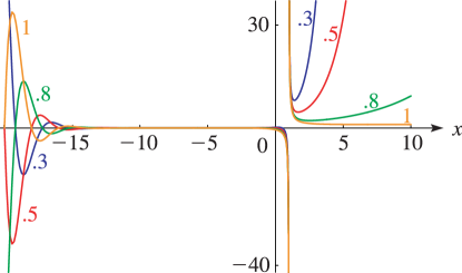
Figure 25.12.2: Absolute value of the dilogarithm function $\left|{\mathrm{Li}}_2\left(x+\mathrm{i}y\right)\right|$, $-20\le x\le 20$, $-20\le y\le 20$. … Magnify 3D Help

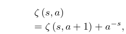
… ►For real or complex $s$ and $z$ the polylogarithm ${\mathrm{Li}}_s\left(z\right)$ is defined by … ►For each fixed complex $s$ the series defines an analytic function of $z$ for . …

9: 7.23 Tables

… ►

§7.23(ii) Real Variables

… ►

§7.23(iii) Complex Variables, $z=x+\mathrm{i}y$

… ►

Zhang and Jin (1996, pp. 638, 640–641) includes the real and imaginary parts of $\mathrm{erf}z$, $x\in [0,5]$, $y=0.5(.5)3$, 7D and 8D, respectively; the real and imaginary parts of ${\int }_x^{\mathrm{\infty }}{\mathrm{e}}^{\pm \mathrm{i}{t}^2}dt$, $(1/\sqrt{\pi }){\mathrm{e}}^{\mp \mathrm{i}(x^2+(\pi /4))}{\int }_x^{\mathrm{\infty }}{\mathrm{e}}^{\pm \mathrm{i}{t}^2}dt$, $x=0(.5)20(1)25$, 8D, together with the corresponding modulus and phase to 8D and 6D (degrees), respectively.

…

10: 30.9 Asymptotic Approximations and Expansions

… ►

$$2^{20}{\beta }_5=-527q^7-61529q^5-\mathrm{10\hspace{0.33em}43961}{q}^3-\mathrm{22\hspace{0.33em}41599}q+32m^2(5739q^5+\mathrm{1\hspace{0.33em}27550}{q}^3+\mathrm{2\hspace{0.33em}98951}q)-2048m^4(355q^3+1505q)+65536m^{6}q.$$

… ►For uniform asymptotic expansions in terms of Airy or Bessel functions for real values of the parameters, complex values of the variable, and with explicit error bounds see Dunster (1986). … ►For uniform asymptotic expansions in terms of elementary, Airy, or Bessel functions for real values of the parameters, complex values of the variable, and with explicit error bounds see Dunster (1992, 1995). … ►The behavior of ${\lambda }_n^m\left({\gamma }^2\right)$ for complex ${\gamma }^2$ and large $|{\lambda }_n^m\left({\gamma }^2\right)|$ is investigated in Hunter and Guerrieri (1982). …