comparison with Clenshaw–Curtis formula

SearchAdvancedHelp

(0.003 seconds)

1—10 of 261 matching pages

1: 3.5 Quadrature

… ►If we add $-1$ and $1$ to this set of $x_k$, then the resulting closed formula is the frequently-used Clenshaw–Curtis formula, whose weights are positive and given by … ►For detailed comparisons of the Clenshaw–Curtis formula with Gauss quadrature (§3.5(v)), see Trefethen (2008, 2011). … ►A comparison of several methods, including an extension of the Clenshaw–Curtis formula (§3.5(iv)), is given in Evans and Webster (1999). …

2: 33.23 Methods of Computation

… ►Curtis (1964a, §10) describes the use of series, radial integration, and other methods to generate the tables listed in §33.24. … ►A set of consistent second-order WKBJ formulas is given by Burgess (1963: in Eq. …

3: Bibliography C

… ►

A method for numerical integration on an automatic copmputer. Numer. Math. 2 (4), pp. 197–205.

ⓘ

External Links:

ISSN 0029-599X, Document, MathReview (A. H. Stroud), ZentralBlatt

Referenced by:

§3.5(iv).

Encodings:

BibTeX

►

Generalized exponential and logarithmic functions. Comput. Math. Appl. Part B 12 (5-6), pp. 1091–1101.

ⓘ

External Links:

ISSN 0886-9561, MathReview (M. E. Muldoon), ZentralBlatt

Referenced by:

§4.12.

Encodings:

BibTeX

►

Algorithms for special functions. I. Numer. Math. 4, pp. 403–419.

ⓘ

External Links:

ISSN 0029-599X, Document, MathReview (A. S. Householder), ZentralBlatt

Referenced by:

§5.24(ii).

Encodings:

BibTeX

►

Level-Index Arithmetic: An Introductory Survey. In Numerical Analysis and Parallel Processing (Lancaster, 1987), P. R. Turner (Ed.), Lecture Notes in Math., Vol. 1397, pp. 95–168.

ⓘ

External Links:

MathReview Entry, ZentralBlatt

Referenced by:

§3.1(iv).

Encodings:

BibTeX

►

Beyond floating point. J. Assoc. Comput. Mach. 31 (2), pp. 319–328.

ⓘ

External Links:

Document, MathReview Entry, ZentralBlatt

Referenced by:

§3.1(iv).

Encodings:

BibTeX

…

4: 28.5 Second Solutions ${\mathrm{fe}}_n$, ${\mathrm{ge}}_n$

… ►(Other normalizations for $C_n(q)$ and $S_n(q)$ can be found in the literature, but most formulas—including connection formulas—are unaffected since ${\mathrm{fe}}_n(z,q)/C_n(q)$ and ${\mathrm{ge}}_n(z,q)/S_n(q)$ are invariant.) … ►

►►

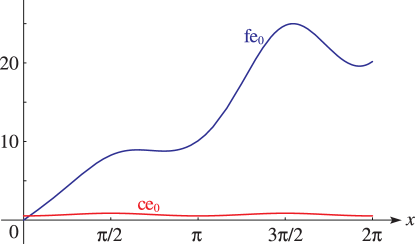
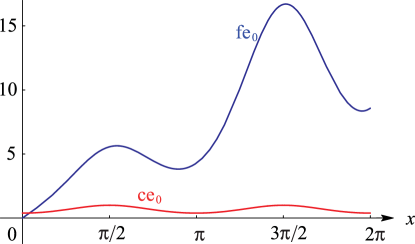
Figure 28.5.1: ${\mathrm{fe}}_0(x,0.5)$ for $0\le x\le 2\pi$ and (for comparison) ${\mathrm{ce}}_0(x,0.5)$. Magnify

►

►►

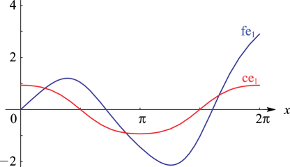
Figure 28.5.2: ${\mathrm{fe}}_0(x,1)$ for $0\le x\le 2\pi$ and (for comparison) ${\mathrm{ce}}_0(x,1)$. Magnify

►

►►

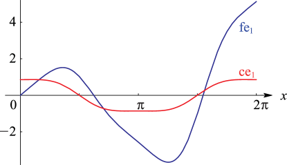
Figure 28.5.3: ${\mathrm{fe}}_1(x,0.5)$ for $0\le x\le 2\pi$ and (for comparison) ${\mathrm{ce}}_1(x,0.5)$. Magnify

►

►►

Figure 28.5.4: ${\mathrm{fe}}_1(x,1)$ for $0\le x\le 2\pi$ and (for comparison) ${\mathrm{ce}}_1(x,1)$. Magnify

…

5: Bibliography R

… ►

Rational Chebyshev approximation by Remes’ algorithms. Numer. Math. 7 (4), pp. 322–330.

ⓘ

External Links:

ISSN 0029-599X, Document, MathReview (C. W. Clenshaw), ZentralBlatt

Referenced by:

§3.11(i).

Encodings:

BibTeX

… ►

Fourier analysis and signal processing by use of the Möbius inversion formula. IEEE Trans. Acoustics, Speech, Signal Processing 38, pp. 458–470.

ⓘ

External Links:

ZentralBlatt

Referenced by:

§27.17.

Encodings:

BibTeX

… ►

Elliptic Integrals of the First and Second Kind – Comparison of Bulirsch’s and Carlson’s Algorithms for Numerical Calculation. In Special Functions (Hong Kong, 1999), C. Dunkl, M. Ismail, and R. Wong (Eds.), pp. 293–308.

ⓘ

External Links:

MathReview, ZentralBlatt

Referenced by:

§19.36(i), §19.36(ii).

Encodings:

BibTeX

… ►

Another proof of the triple sum formula for Wigner $9j$-symbols. J. Math. Phys. 40 (12), pp. 6689–6691.

ⓘ

External Links:

ISSN 0022-2488, Document, MathReview (Michael Wüstner), ZentralBlatt

Referenced by:

§34.6.

Encodings:

BibTeX

…

6: 18.40 Methods of Computation

… ►For applications in which the OP’s appear only as terms in series expansions (compare §18.18(i)) the need to compute them can be avoided altogether by use instead of Clenshaw’s algorithm (§3.11(ii)) and its straightforward generalization to OP’s other than Chebyshev. For further information see Clenshaw (1955), Gautschi (2004, §§2.1, 8.1), and Mason and Handscomb (2003, §2.4). … ►Comparisons of the precisions of Lagrange and PWCF interpolations to obtain the derivatives, are shown in Figure 18.40.2. …

7: 2.10 Sums and Sequences

… ►

§2.10(i) Euler–Maclaurin Formula

… ►Another version is the Abel–Plana formula: … ►We need a “comparison function” $g(z)$ with the properties: … ►

The coefficients in the Laurent expansion

2.10.27 $$g(z)=\sum _{n=-\mathrm{\infty }}^{\mathrm{\infty }}{g}_n{z}^n,$$ ,

ⓘ

Symbols:

$r$: radious of annulus, $g(z)$: comparison function and $g_n$: coefficients

Permalink:

http://dlmf.nist.gov/2.10.E27

Encodings:

pMML, png, TeX

See also:

Annotations for §2.10(iv), §2.10 and Ch.2

have known asymptotic behavior as $n\to \pm \mathrm{\infty }$.

… ►

On the circle $|z|=r$, the function $f(z)-g(z)$ has a finite number of singularities, and at each singularity $z_j$, say,

2.10.30 $$f(z)-g(z)=O\left({(z-z_j)}^{{\sigma }_j-1}\right),$$ $z\to z_j$,

ⓘ

Symbols:

$O\left(x\right)$: order not exceeding, $f(x)$: analytic function, $g(z)$: comparison function and ${\sigma }_j$: positive constant

Permalink:

http://dlmf.nist.gov/2.10.E30

Encodings:

pMML, png, TeX

See also:

Annotations for §2.10(iv), §2.10 and Ch.2

where ${\sigma }_j$ is a positive constant.

…

8: Bibliography W

… ►

Fast construction of the Fejér and Clenshaw-Curtis quadrature rules. BIT 46 (1), pp. 195–202.

ⓘ

External Links:

ISSN 0006-3835, Document, MathReview Entry, ZentralBlatt

Referenced by:

§3.5(iv).

Encodings:

BibTeX

… ►

Reduction formulae for products of theta functions. J. Res. Nat. Inst. Standards and Technology 117, pp. 297–303.

ⓘ

External Links:

Document

Referenced by:

(20.7.34), §20.7(ix).

Encodings:

BibTeX

… ►

Rational Chebyshev approximations for the Bessel functions $J_0(x)$, $J_1(x)$, $Y_0(x)$, $Y_1(x)$ . Math. Comp. 39 (160), pp. 617–623.

ⓘ

Notes:

Tables on microfiche

External Links:

ISSN 0025-5718, FullText, MathReview (C. W. Clenshaw), ZentralBlatt

Referenced by:

9th item.

Encodings:

BibTeX

… ►

Recursion formulae for hypergeometric functions. Math. Comp. 22 (102), pp. 363–373.

ⓘ

External Links:

FullText, Document, MathReview (S. D. Bajpai), ZentralBlatt

Referenced by:

§16.3(ii).

Encodings:

BibTeX

… ►

Quadrature formulas for oscillatory integral transforms. Numer. Math. 39 (3), pp. 351–360.

ⓘ

External Links:

ISSN 0029-599X, Document, MathReview (A.J. Rodrigues), ZentralBlatt

Referenced by:

§10.74(vii), §3.5(vii).

Encodings:

BibTeX

…

9: Bibliography P

… ►

An asymptotic formula for the incomplete gamma function. Ž. Vyčisl. Mat. i Mat. Fiz. 5, pp. 118–121 (Russian).

ⓘ

Notes:

English translation in U.S.S.R. Computational Math. and Math. Phys. 5(1), pp. 162–166

External Links:

Document, MathReview (E. Lukacs), ZentralBlatt

Referenced by:

§8.11(iv).

Encodings:

BibTeX

… ►

Modified Clenshaw-Curtis method for the computation of Bessel function integrals. BIT 23 (3), pp. 370–381.

ⓘ

External Links:

ISSN 0006-3835, Document, MathReview (H. E. Fettis), ZentralBlatt

Referenced by:

§10.74(vii).

Encodings:

BibTeX

… ►

Fast analytic formulas for the modified Bessel functions of imaginary order for spectral line broadening calculations. J. Quantit. Spec. and Rad. Trans. 62 (4), pp. 389–395.

ⓘ

External Links:

Document

Referenced by:

§10.76(ii).

Encodings:

BibTeX

… ►

Recurrence formulas for Coulomb wave functions. Physical Rev. (2) 72 (7), pp. 626–627.

ⓘ

External Links:

Document, MathReview (S. C. van Veen), ZentralBlatt

Referenced by:

§33.4.

Encodings:

BibTeX

…

10: 29.20 Methods of Computation

… ►Subsequently, formulas typified by (29.6.4) can be applied to compute the coefficients of the Fourier expansions of the corresponding Lamé functions by backward recursion followed by application of formulas typified by (29.6.5) and (29.6.6) to achieve normalization; compare §3.6. …The Fourier series may be summed using Clenshaw’s algorithm; see §3.11(ii). … ►§29.15(i) includes formulas for normalizing the eigenvectors. …