coefficients

SearchAdvancedHelp

(0.001 seconds)

1—10 of 241 matching pages

1: 26.3 Lattice Paths: Binomial Coefficients

§26.3 Lattice Paths: Binomial Coefficients

►

§26.3(i) Definitions

… ►

§26.3(ii) Generating Functions

… ►

§26.3(iii) Recurrence Relations

… ►

§26.3(iv) Identities

…

2: 26.21 Tables

§26.21 Tables

►Abramowitz and Stegun (1964, Chapter 24) tabulates binomial coefficients $\left(\genfrac{}{}{0.0pt}{}{m}{n}\right)$ for $m$ up to 50 and $n$ up to 25; extends Table 26.4.1 to $n=10$; tabulates Stirling numbers of the first and second kinds, $s(n,k)$ and $S(n,k)$, for $n$ up to 25 and $k$ up to $n$; tabulates partitions $p\left(n\right)$ and partitions into distinct parts $p(𝒟,n)$ for $n$ up to 500. … ►Goldberg et al. (1976) contains tables of binomial coefficients to $n=100$ and Stirling numbers to $n=40$.

3: 28.14 Fourier Series

… ►The coefficients satisfy ►

28.14.4 $$q{c}_{2m+2}-\left(a-{(\nu +2m)}^2\right)c_{2m}+q{c}_{2m-2}=0,$$ $a={\lambda }_{\nu }\left(q\right),c_{2m}=c_{2m}^{\nu }(q)$,

ⓘ

Symbols:

${\lambda }_{\nu +2n}\left(q\right)$: eigenvalues of Mathieu equation, $m$: integer, $q=h^2$: parameter, $\nu$: complex parameter, $a$: parameter and $c_{2m}(q)$: coefficients

Referenced by:

item (d), item (d)

Permalink:

http://dlmf.nist.gov/28.14.E4

Encodings:

pMML, png, TeX

See also:

Annotations for §28.14 and Ch.28

… ►

28.14.5 $$\sum _{m=-\mathrm{\infty }}^{\mathrm{\infty }}{\left(c_{2m}^{\nu }(q)\right)}^2=1;$$

ⓘ

Symbols:

$m$: integer, $q=h^2$: parameter, $\nu$: complex parameter and $c_{2m}(q)$: coefficients

Referenced by:

item (d)

Permalink:

http://dlmf.nist.gov/28.14.E5

Encodings:

pMML, png, TeX

See also:

Annotations for §28.14 and Ch.28

… ►

28.14.7 $$c_{-2m}^{-\nu }(q)=c_{2m}^{\nu }(q),$$

ⓘ

Symbols:

$m$: integer, $q=h^2$: parameter, $\nu$: complex parameter and $c_{2m}(q)$: coefficients

Permalink:

http://dlmf.nist.gov/28.14.E7

Encodings:

pMML, png, TeX

See also:

Annotations for §28.14 and Ch.28

►

28.14.8 $$c_{2m}^{\nu }(-q)={(-1)}^m{c}_{2m}^{\nu }(q).$$

ⓘ

Symbols:

$m$: integer, $q=h^2$: parameter, $\nu$: complex parameter and $c_{2m}(q)$: coefficients

Permalink:

http://dlmf.nist.gov/28.14.E8

Encodings:

pMML, png, TeX

See also:

Annotations for §28.14 and Ch.28

…

4: 26.4 Lattice Paths: Multinomial Coefficients and Set Partitions

§26.4 Lattice Paths: Multinomial Coefficients and Set Partitions

►

§26.4(i) Definitions

… ► $M_1$ is the multinominal coefficient (26.4.2): … ►

§26.4(ii) Generating Function

… ►

§26.4(iii) Recurrence Relation

…

5: 29.20 Methods of Computation

… ►Subsequently, formulas typified by (29.6.4) can be applied to compute the coefficients of the Fourier expansions of the corresponding Lamé functions by backward recursion followed by application of formulas typified by (29.6.5) and (29.6.6) to achieve normalization; compare §3.6. … ►A third method is to approximate eigenvalues and Fourier coefficients of Lamé functions by eigenvalues and eigenvectors of finite matrices using the methods of §§3.2(vi) and 3.8(iv). …The approximations converge geometrically (§3.8(i)) to the eigenvalues and coefficients of Lamé functions as $n\to \mathrm{\infty }$. … ►

§29.20(ii) Lamé Polynomials

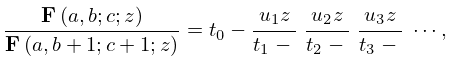
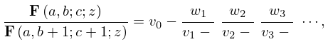
… ►The corresponding eigenvectors yield the coefficients in the finite Fourier series for Lamé polynomials. …

6: 15.7 Continued Fractions

… ►

15.7.1 $$\frac{𝐅(a,b;c;z)}{𝐅(a,b+1;c+1;z)}=t_0-\frac{u_{1}z}{t_1-}\frac{u_{2}z}{t_2-}\frac{u_{3}z}{t_3-}\mathrm{\cdots },$$

ⓘ

Symbols:

$𝐅(a,b;c;z)$ or $𝐅(\genfrac{}{}{0pt}{}{a,b}{c};z)$: $={}_2{}^{}𝐅_1^{}(a,b;c;z)$ Olver’s hypergeometric function, $z$: complex variable, $a$: real or complex parameter, $b$: real or complex parameter, $c$: real or complex parameter, $t_n$: coefficient and $u_n$: coefficient

Permalink:

http://dlmf.nist.gov/15.7.E1

Encodings:

pMML, png, TeX

See also:

Annotations for §15.7 and Ch.15

►where … ►

15.7.3 $$\frac{𝐅(a,b;c;z)}{𝐅(a,b+1;c+1;z)}=v_0-\frac{w_1}{v_1-}\frac{w_2}{v_2-}\frac{w_3}{v_3-}\mathrm{\cdots },$$

ⓘ

Symbols:

$𝐅(a,b;c;z)$ or $𝐅(\genfrac{}{}{0pt}{}{a,b}{c};z)$: $={}_2{}^{}𝐅_1^{}(a,b;c;z)$ Olver’s hypergeometric function, $z$: complex variable, $a$: real or complex parameter, $b$: real or complex parameter, $c$: real or complex parameter, $v_n$: coefficient and $w_n$: coefficient

Permalink:

http://dlmf.nist.gov/15.7.E3

Encodings:

pMML, png, TeX

See also:

Annotations for §15.7 and Ch.15

►where …

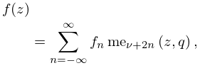
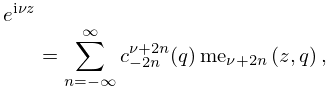
7: 28.4 Fourier Series

… ►

§28.4(ii) Recurrence Relations

… ►

§28.4(iii) Normalization

… ►

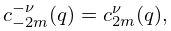
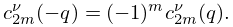
§28.4(v) Change of Sign of $q$

… ►

§28.4(vi) Behavior for Small $q$

… ►

§28.4(vii) Asymptotic Forms for Large $m$

…

8: 29.21 Tables

… ►

Arscott and Khabaza (1962) tabulates the coefficients of the polynomials $P$ in Table 29.12.1 (normalized so that the numerically largest coefficient is unity, i.e. monic polynomials), and the corresponding eigenvalues $h$ for $k^2=0.1(.1)0.9$, $n=1(1)30$. Equations from §29.6 can be used to transform to the normalization adopted in this chapter. Precision is 6S.

9: 34.1 Special Notation

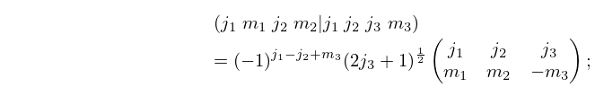
… ►An often used alternative to the $\mathit{3}j$ symbol is the Clebsch–Gordan coefficient ►

34.1.1

ⓘ

Symbols:

: $\mathit{3}j$ symbol and $j,j_r$: non-negative integers or non-negative integers plus one half.

Sources:

Edmonds (1974, p. 46, Eq. (3.7.3)); Rotenberg et al. (1959, p. 1, Eq. (1.1a))

Permalink:

http://dlmf.nist.gov/34.1.E1

Encodings:

pMML, png, TeX

Clarification (effective with 1.0.15):

A wording change reflects that the Clebsch–Gordan coefficients are an alternative formulation of angular momentum problems, rather than alternative notation for the $\mathit{3}j$. The sign of $m_3$ was changed for clarity.

See also:

Annotations for §34.1 and Ch.34

… ►For other notations for $\mathit{3}j$, $\mathit{6}j$, $\mathit{9}j$ symbols, see Edmonds (1974, pp. 52, 97, 104–105) and Varshalovich et al. (1988, §§8.11, 9.10, 10.10).

10: 28.19 Expansions in Series of ${\mathrm{me}}_{\nu +2n}$ Functions

… ►

28.19.2 $$f(z)=\sum _{n=-\mathrm{\infty }}^{\mathrm{\infty }}{f}_n{\mathrm{me}}_{\nu +2n}(z,q),$$

ⓘ

Defines:

$f(z)$: function (locally)

Symbols:

${\mathrm{me}}_n(z,q)$: Mathieu function, $q=h^2$: parameter, $n$: integer, $z$: complex variable, $\nu$: complex parameter and $f_n$: coefficients

Referenced by:

§28.19

Permalink:

http://dlmf.nist.gov/28.19.E2

Encodings:

pMML, png, TeX

See also:

Annotations for §28.19 and Ch.28

… ►

28.19.3 $$f_n=\frac{1}{\pi }{\int }_0^{\pi }f(z){\mathrm{me}}_{\nu +2n}(-z,q)dz.$$

ⓘ

Defines:

$f_n$: coefficients (locally)

Symbols:

${\mathrm{me}}_n(z,q)$: Mathieu function, $\pi$: the ratio of the circumference of a circle to its diameter, $dx$: differential of $x$ , $\int$: integral, $q=h^2$: parameter, $n$: integer, $z$: complex variable, $\nu$: complex parameter and $f(z)$: function

Permalink:

http://dlmf.nist.gov/28.19.E3

Encodings:

pMML, png, TeX

See also:

Annotations for §28.19 and Ch.28

… ►

28.19.4 $${\mathrm{e}}^{\mathrm{i}\nu z}=\sum _{n=-\mathrm{\infty }}^{\mathrm{\infty }}{c}_{-2n}^{\nu +2n}(q){\mathrm{me}}_{\nu +2n}(z,q),$$

ⓘ

Symbols:

${\mathrm{me}}_n(z,q)$: Mathieu function, $\mathrm{e}$: base of natural logarithm, $\mathrm{i}$: imaginary unit, $q=h^2$: parameter, $n$: integer, $z$: complex variable, $\nu$: complex parameter and $c_{2m}(q)$: coefficients

Permalink:

http://dlmf.nist.gov/28.19.E4

Encodings:

pMML, png, TeX

See also:

Annotations for §28.19, §28.19 and Ch.28

►where the coefficients are as in §28.14.