closure

(0.000 seconds)

9 matching pages

1: 1.4 Calculus of One Variable

… ►A generalization of the Riemann integral is the Stieltjes integral

\int_{a}^{b}f(x)\,\mathrm{d}\alpha(x)

, where

\alpha(x)

is a nondecreasing function on the closure of

(a,b)

, which may be bounded, or unbounded, and

\,\mathrm{d}\alpha(x)

is the Stieltjes measure. … ►For

\alpha(x)

nondecreasing on the closure

I

of an interval

(a,b)

, the measure

\,\mathrm{d}\alpha

is absolutely continuous if

\alpha(x)

is continuous and there exists a weight function

w(x)\geq 0

, Riemann (or Lebesgue) integrable on finite subintervals of

I

, such that … ►where the supremum is over all sets of points

x_{0}<x_{1}<\cdots<x_{n}

in the closure of

(a,b)

, that is,

(a,b)

with

a, b

added when they are finite. … ►If

f(x)

is continuous on the closure of

(a,b)

and

f^{\prime}(x)

is continuous on

(a,b)

, then …

2: 13.9 Zeros

… ►Let

P_{\alpha}

denote the closure of the domain that is bounded by the parabola

y^{2}=4\alpha(x+\alpha)

and contains the origin. …

3: 3.7 Ordinary Differential Equations

… ►Let

(a,b)

be a finite or infinite interval and

q(x)

be a real-valued continuous (or piecewise continuous) function on the closure of

(a,b)

. … ►If

q(x)

C^{\infty}

on the closure of

(a,b)

, then the discretized form (3.7.13) of the differential equation can be used. …

4: 1.9 Calculus of a Complex Variable

… ►Also, the union of

S

and its limit points is the closure of

S

. …

5: 13.7 Asymptotic Expansions for Large Argument

… ►

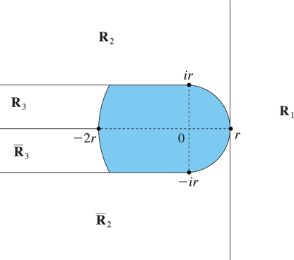
See accompanying text — Figure 13.7.1: Regions ${\textbf{R}}_{1}$ , ${\textbf{R}}_{2}$ , $\overline{\textbf{R}}_{2}$ , ${\textbf{R}}_{3}$ , and $\overline{\textbf{R}}_{3}$ are the closures of the indicated unshaded regions bounded by the straight lines and circular arcs centered at the origin, with $r=|b-2a|$ . Magnify

…

6: 18.2 General Orthogonal Polynomials

… ►It is assumed throughout this chapter that for each polynomial

p_{n}(x)

that is orthogonal on an open interval

(a,b)

the variable

x

is confined to the closure of

(a,b)

unless indicated otherwise. (However, under appropriate conditions almost all equations given in the chapter can be continued analytically to various complex values of the variables.) … ►More generally than (18.2.1)–(18.2.3),

w(x)\,\mathrm{d}x

may be replaced in (18.2.1) by

\,\mathrm{d}\mu(x)

, where the measure

\mu

is the Lebesgue–Stieltjes measure

\mu_{\alpha}

corresponding to a bounded nondecreasing function

\alpha

on the closure of

(a,b)

with an infinite number of points of increase, and such that

\int_{a}^{b}|x|^{n}\,\mathrm{d}\mu(x)<\infty

for all

n

. …

7: 2.10 Sums and Sequences

… ►

(a)

On the strip $a\leq\Re z\leq n$ , $f(z)$ is analytic in its interior, $f^{(2m)}(z)$ is continuous on its closure, and $f(z)=o\left(e^{2\pi|\Im z|}\right)$ as $\Im z\to\pm\infty$ , uniformly with respect to $\Re z\in[a,n]$ .

…

8: 1.16 Distributions

… ►The closure of the set of points where

\phi\not=0

is called the support of

\phi

. …

9: 18.18 Sums

… ►In this subsection the variables

x

and

y

are not confined to the closures of the intervals of orthogonality; compare §18.2(i). …