circular%20cases

(0.002 seconds)

1—10 of 11 matching pages

1: 36.2 Catastrophes and Canonical Integrals

… ►Special cases:

K=1

, fold catastrophe;

K=2

, cusp catastrophe;

K=3

, swallowtail catastrophe. … ►

§36.2(ii) Special Cases

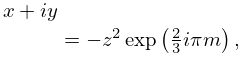
… ►Addendum: For further special cases see §36.2(iv) … ►(rotation by

\pm\tfrac{2}{3}\pi

x, y

plane). … ►

§36.2(iv) Addendum to 36.2(ii) Special Cases

…

2: 20.7 Identities

… ►

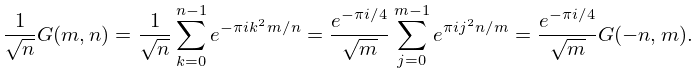
20.7.22

\theta_{2}\left(4z\middle|4\tau\right)=B\theta_{2}\left(\tfrac{1}{8}\pi-z% \middle|\tau\right)\theta_{2}\left(\tfrac{1}{8}\pi+z\middle|\tau\right)\*% \theta_{2}\left(\tfrac{3}{8}\pi-z\middle|\tau\right)\theta_{2}\left(\tfrac{3}{% 8}\pi+z\middle|\tau\right),

ⓘ

Symbols:: $\theta_{\NVar{j}}\left(\NVar{z}\middle|\NVar{\tau}\right)$ : theta function, $\pi$ : the ratio of the circumference of a circle to its diameter, $z$ : complex, $\tau$ : lattice parameter and $B$
Permalink:: http://dlmf.nist.gov/20.7.E22
Encodings:: pMML, png, TeX
See also:: Annotations for §20.7(vi), §20.7 and Ch.20

►

20.7.23

\theta_{3}\left(4z\middle|4\tau\right)=B\theta_{3}\left(\tfrac{1}{8}\pi-z% \middle|\tau\right)\theta_{3}\left(\tfrac{1}{8}\pi+z\middle|\tau\right)\*% \theta_{3}\left(\tfrac{3}{8}\pi-z\middle|\tau\right)\theta_{3}\left(\tfrac{3}{% 8}\pi+z\middle|\tau\right),

ⓘ

Symbols:: $\theta_{\NVar{j}}\left(\NVar{z}\middle|\NVar{\tau}\right)$ : theta function, $\pi$ : the ratio of the circumference of a circle to its diameter, $z$ : complex, $\tau$ : lattice parameter and $B$
Permalink:: http://dlmf.nist.gov/20.7.E23
Encodings:: pMML, png, TeX
See also:: Annotations for §20.7(vi), §20.7 and Ch.20

… ►See Lawden (1989, pp. 19–20). … ►These are specific examples of modular transformations as discussed in §23.15; the corresponding results for the general case are given by Rademacher (1973, pp. 181–183). … ►

20.7.34

\frac{\theta_{1}\left(z,q^{2}\right)\theta_{3}\left(z,q^{2}\right)}{\theta_{1}% \left(z,iq\right)}=\frac{\theta_{2}\left(z,q^{2}\right)\theta_{4}\left(z,q^{2}% \right)}{\theta_{2}\left(z,iq\right)}=i^{-1/4}\sqrt{\frac{\theta_{2}\left(0,q^% {2}\right)\theta_{4}\left(0,q^{2}\right)}{2}}.

ⓘ

Symbols:: $\theta_{\NVar{j}}\left(\NVar{z},\NVar{q}\right)$ : theta function, $\mathrm{i}$ : imaginary unit, $z$ : complex and $q$ : nome
Referenced by:: §20.7(iv), Erratum (V1.0.5) for Chapters 8, 20, 36
Permalink:: http://dlmf.nist.gov/20.7.E34
Encodings:: pMML, png, TeX
Addition (effective with 1.0.5):: This equation has been added. See Walker (2012).
See also:: Annotations for §20.7(ix), §20.7 and Ch.20

…

3: 19.36 Methods of Computation

… ►The computation is slowest for complete cases. … ►Complete cases of Legendre’s integrals and symmetric integrals can be computed with quadratic convergence by the AGM method (including Bartky transformations), using the equations in §19.8(i) and §19.22(ii), respectively. … ►The step from

n

n+1

is an ascending Landen transformation if

\theta=1

(leading ultimately to a hyperbolic case of

R_{C}

) or a descending Gauss transformation if

\theta=-1

(leading to a circular case of

R_{C}

). … ►Also, see Todd (1975) for a special case of

K\left(k\right)

. For computation of Legendre’s integral of the third kind, see Abramowitz and Stegun (1964, §§17.7 and 17.8, Examples 15, 17, 19, and 20). …

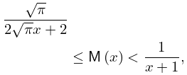
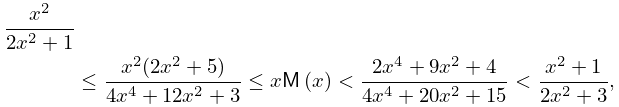
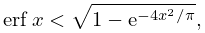
4: 7.8 Inequalities

… ►

7.8.2

\frac{1}{x+\sqrt{x^{2}+2}}<\mathsf{M}\left(x\right)\leq\frac{1}{x+\sqrt{x^{2}+% (4/\pi)}},

x\geq 0

ⓘ

Symbols:: $\mathsf{M}\left(\NVar{x}\right)$ : Mills’ ratio, $\pi$ : the ratio of the circumference of a circle to its diameter and $x$ : real variable
A&S Ref:: 7.1.13
Referenced by:: §7.8
Permalink:: http://dlmf.nist.gov/7.8.E2
Encodings:: pMML, png, TeX
See also:: Annotations for §7.8 and Ch.7

►

7.8.3

\frac{\sqrt{\pi}}{2\sqrt{\pi}x+2}\leq\mathsf{M}\left(x\right)<\frac{1}{x+1},

x\geq 0

ⓘ

Symbols:: $\mathsf{M}\left(\NVar{x}\right)$ : Mills’ ratio, $\pi$ : the ratio of the circumference of a circle to its diameter and $x$ : real variable
Referenced by:: §7.8
Permalink:: http://dlmf.nist.gov/7.8.E3
Encodings:: pMML, png, TeX
See also:: Annotations for §7.8 and Ch.7

… ►

7.8.5

\frac{x^{2}}{2x^{2}+1}\leq\frac{x^{2}(2x^{2}+5)}{4x^{4}+12x^{2}+3}\leq x% \mathsf{M}\left(x\right)<\frac{2x^{4}+9x^{2}+4}{4x^{4}+20x^{2}+15}<\frac{x^{2}% +1}{2x^{2}+3},

x\geq 0

ⓘ

Symbols:: $\mathsf{M}\left(\NVar{x}\right)$ : Mills’ ratio and $x$ : real variable
Referenced by:: §7.8
Permalink:: http://dlmf.nist.gov/7.8.E5
Encodings:: pMML, png, TeX
See also:: Annotations for §7.8 and Ch.7

… ►

7.8.8

\operatorname{erf}x<\sqrt{1-{\mathrm{e}}^{-4x^{2}/\pi}},

x>0

ⓘ

Symbols:: $\pi$ : the ratio of the circumference of a circle to its diameter, $\operatorname{erf}\NVar{z}$ : error function, $\mathrm{e}$ : base of natural logarithm and $x$ : real variable
Source:: Pólya (1949, (1.5))
Referenced by:: §7.8, Erratum (V1.0.17) for Equation (7.8.8)
Permalink:: http://dlmf.nist.gov/7.8.E8
Encodings:: pMML, png, TeX
Addition (effective with 1.0.17):: This inequality was added. It is Pólya (1949, (1.5)). Note that it is a special case of (8.10.11).
Suggested by Roberto Iacono
See also:: Annotations for §7.8 and Ch.7

5: 25.12 Polylogarithms

… ►When

z=e^{i\theta}

0\leq\theta\leq 2\pi

, (25.12.1) becomes … ►The special case

z=1

is the Riemann zeta function:

\zeta\left(s\right)=\operatorname{Li}_{s}\left(1\right)

. … ►valid when

\Re s>0

and

\left|\operatorname{ph}\left(1-z\right)\right|<\pi

, or

\Re s>1

and

z=1

. (In the latter case (25.12.11) becomes (25.5.1)). … ►When

s=2

and

e^{2\pi ia}=z

, (25.12.13) becomes (25.12.4). …

6: 36.4 Bifurcation Sets

… ►

Special Cases

… ►

x=\tfrac{9}{20}z^{2}.

… ►

x=-\tfrac{3}{20}z^{2},

… ►

y=\tfrac{1}{3}z^{2}(\sin\left(2\phi\right)-2\sin\phi)

0\leq\phi\leq 2\pi

… ►

36.4.11

x+iy=-z^{2}\exp\left(\tfrac{2}{3}i\pi m\right),

m=0,1,2

ⓘ

Symbols:: $\pi$ : the ratio of the circumference of a circle to its diameter, $\exp\NVar{z}$ : exponential function, $\mathrm{i}$ : imaginary unit, $y$ : real parameter, $z$ : real parameter, $n$ : integer and $x$ : real parameter
Referenced by:: §36.7(iii)
Permalink:: http://dlmf.nist.gov/36.4.E11
Encodings:: pMML, png, TeX
See also:: Annotations for §36.4(i), §36.4(i), §36.4 and Ch.36

…

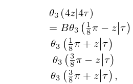
7: 20.11 Generalizations and Analogs

… ►

20.11.2

\frac{1}{\sqrt{n}}G(m,n)=\frac{1}{\sqrt{n}}\sum\limits_{k=0}^{n-1}e^{-\pi ik^{% 2}m/n}=\frac{e^{-\pi i/4}}{\sqrt{m}}\sum\limits_{j=0}^{m-1}e^{\pi ij^{2}n/m}=% \frac{e^{-\pi i/4}}{\sqrt{m}}G(-n,m).

ⓘ

Symbols:: $\pi$ : the ratio of the circumference of a circle to its diameter, $\mathrm{e}$ : base of natural logarithm, $\mathrm{i}$ : imaginary unit, $m$ : integer, $n$ : integer and $G(m,n)$ : Gauss sum
Permalink:: http://dlmf.nist.gov/20.11.E2
Encodings:: pMML, png, TeX
See also:: Annotations for §20.11(i), §20.11 and Ch.20

… ►With the substitutions

a=qe^{2iz}

b=qe^{-2iz}

, with

q=e^{i\pi\tau}

, we have … ►In the case

z=0

identities for theta functions become identities in the complex variable

q

, with

\left|q\right|<1

, that involve rational functions, power series, and continued fractions; see Adiga et al. (1985), McKean and Moll (1999, pp. 156–158), and Andrews et al. (1988, §10.7). … ►However, in this case

q

is no longer regarded as an independent complex variable within the unit circle, because

k

is related to the variable

\tau=\tau(k)

of the theta functions via (20.9.2). … ►For applications to rapidly convergent expansions for

\pi

see Chudnovsky and Chudnovsky (1988), and for applications in the construction of elliptic-hypergeometric series see Rosengren (2004). …

8: 12.11 Zeros

… ►Lastly, when

a=-n-\tfrac{1}{2}

n=1,2,\dots

(Hermite polynomial case)

U\left(a,x\right)

has

n

zeros and they lie in the interval

[-2\sqrt{-a},2\sqrt{-a}\,]

. For further information on these cases see Dean (1966). … ►When

a>-\frac{1}{2}

U\left(a,z\right)

has a string of complex zeros that approaches the ray

\operatorname{ph}z=\frac{3}{4}\pi

z\to\infty

, and a conjugate string. … ►Numerical calculations in this case show that

z_{\frac{1}{2},s}

corresponds to the

s

th zero on the string; compare §7.13(ii). … ►

12.11.9

u_{a,1}\sim 2^{\frac{1}{2}}\mu\left(1-1.85575\;708\mu^{-4/3}-0.34438\;34\mu^{-% 8/3}-0.16871\;5\mu^{-4}-0.11414\mu^{-16/3}-0.0808\mu^{-20/3}-\cdots\right),

ⓘ

Symbols:: $\sim$ : Poincaré asymptotic expansion, $a$ : real or complex parameter and $u_{a,s}$ : zeros
Referenced by:: §12.11(iii)
Permalink:: http://dlmf.nist.gov/12.11.E9
Encodings:: pMML, png, TeX
See also:: Annotations for §12.11(iii), §12.11 and Ch.12

…

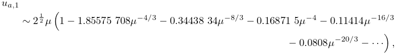
9: 5.11 Asymptotic Expansions

… ►As

z\to\infty

in the sector

|\operatorname{ph}z|\leq\pi-\delta

, … ►Wrench (1968) gives exact values of

g_{k}

up to

g_{20}

. … ►In the case

K=1

the factor

1+\zeta\left(K\right)

is replaced with 4. For this result and a similar bound for the sector

\frac{1}{2}\pi\leq\operatorname{ph}z\leq\pi

see Boyd (1994). … ►For the error term in (5.11.19) in the case

z=x\;(>0)

and

c=1

, see Olver (1995). …

10: Bibliography M

… ►

A. J. MacLeod (1996b) Rational approximations, software and test methods for sine and cosine integrals. Numer. Algorithms 12 (3-4), pp. 259–272.

ⓘ

Notes:: Includes Fortran code, maximum accuracy 20S.
External Links:: ISSN 1017-1398, Document, MathReview, ZentralBlatt
Referenced by:: §6.13, 4th item, §6.21(ii).
Encodings:: BibTeX

… ►

H. R. McFarland and D. St. P. Richards (2001) Exact misclassification probabilities for plug-in normal quadratic discriminant functions. I. The equal-means case. J. Multivariate Anal. 77 (1), pp. 21–53.

ⓘ

External Links:: ISSN 0047-259X, Document, MathReview (Peter A. Lachenbruch), ZentralBlatt
Referenced by:: §35.9.
Encodings:: BibTeX

… ►

Fr. Mechel (1966) Calculation of the modified Bessel functions of the second kind with complex argument. Math. Comp. 20 (95), pp. 407–412.

ⓘ

External Links:: ISSN 0025-5718, FullText, MathReview (H. E. Fettis), ZentralBlatt
Referenced by:: §10.74(iii).
Encodings:: BibTeX

… ►

R. Metzler, J. Klafter, and J. Jortner (1999) Hierarchies and logarithmic oscillations in the temporal relaxation patterns of proteins and other complex systems. Proc. Nat. Acad. Sci. U .S. A. 96 (20), pp. 11085–11089.

ⓘ

External Links:: FullText
Referenced by:: §8.24(i).
Encodings:: BibTeX

… ►

D. S. Moak (1981) The

q

-analogue of the Laguerre polynomials. J. Math. Anal. Appl. 81 (1), pp. 20–47.

ⓘ

External Links:: ISSN 0022-247X, Document, MathReview (R. A. Askey), ZentralBlatt
Referenced by:: §18.27(v).
Encodings:: BibTeX

…