change of order of integration
(0.002 seconds)
11—20 of 20 matching pages
11: 2.11 Remainder Terms; Stokes Phenomenon
…
►By integration by parts (§2.3(i))
…
►That the change in their forms is discontinuous, even though the function being approximated is analytic, is an example of the Stokes
phenomenon.
Where should the change-over take place? Can it be accomplished smoothly?
…
►For higher-order Stokes phenomena see Olde Daalhuis (2004b) and Howls et al. (2004).
…
►For higher-order differential equations, see Olde Daalhuis (1998a, b).
…
12: 19.25 Relations to Other Functions
…
►then the five nontrivial permutations of that leave invariant change
() into , , , , , and () into , , , , .
…
►The three changes of parameter of in §19.7(iii) are unified in (19.21.12) by way of (19.25.14).
…
►The sign on the right-hand side of (19.25.35) will change whenever one crosses a curve on which , for some .
…
►The sign on the right-hand side of (19.25.40) will change whenever one crosses a curve on which , for some .
…
13: 3.5 Quadrature
§3.5 Quadrature
… ►§3.5(iii) Romberg Integration
►Further refinements are achieved by Romberg integration. … ►For these cases the integration path may need to be deformed; see §3.5(ix). … ►With function values, the Monte Carlo method aims at an error of order , independently of the dimension of the domain of integration. …14: 3.7 Ordinary Differential Equations
…
►Consideration will be limited to ordinary linear second-order
differential equations
…
►( and being the identity and zero matrices of order
.)
…
►
First-Order Equations
►For the standard fourth-order rule reads … ►Second-Order Equations
…15: Bibliography B
…
►
Algebro-geometric Approach to Nonlinear Integrable Problems.
Springer Series in Nonlinear Dynamics, Springer-Verlag, Berlin.
…
►
A general program to calculate atomic continuum processes using the R-matrix method.
Comput. Phys. Comm. 8 (3), pp. 149–198.
…
►
Approximating the matrix Fisher and Bingham distributions: Applications to spherical regression and Procrustes analysis.
J. Multivariate Anal. 41 (2), pp. 314–337.
…
►
Constant mean curvature surfaces and integrable equations.
Uspekhi Mat. Nauk 46 (4(280)), pp. 3–42, 192 (Russian).
…
►
Integrable Hamiltonian systems and the Painlevé property.
Phys. Rev. A (3) 25 (3), pp. 1257–1264.
…
16: 1.18 Linear Second Order Differential Operators and Eigenfunction Expansions
§1.18 Linear Second Order Differential Operators and Eigenfunction Expansions
… ►We integrate by parts twice giving: … ►§1.18(iv) Formally Self-adjoint Linear Second Order Differential Operators
… ►In general, operators being formally self-adjoint second order differential operators of the form (1.18.28), with unbounded, will have both a continuous and a point spectrum, and thus, correspondingly, eigenfunctions as in §1.18(vi) and eigenfunctions as in §1.18(v). … ►For a formally self-adjoint second order differential operator , such as that of (1.18.28), the space can be seen to consist of all such that the distribution can be identified with a function in , which is the function . …17: 2.8 Differential Equations with a Parameter
…
►For example, can be the order of a Bessel function or degree of an orthogonal polynomial.
…
►This introduces new variables and , related by
…
►(the constants of integration being arbitrary).
…
►
§2.8(iv) Case III: Simple Pole
… ►Lastly, for an example of a fourth-order differential equation, see Wong and Zhang (2007). …18: 1.10 Functions of a Complex Variable
…
►and the integration contour is described once in the positive sense.
…
►If is the first negative integer (counting from ) with , then is a pole of order (or multiplicity) .
…
►where and are respectively the numbers of zeros and poles, counting multiplicity, of within , and is the change in any continuous branch of as passes once around in the positive sense.
…
►(For example, when is an integer has a zero of order
at .)
…
►is analytic in and its derivatives of all orders can be found by differentiating under the sign of integration.
…
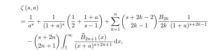
19: 25.11 Hurwitz Zeta Function
…
►
25.11.7
, , , .
…
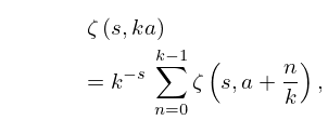
►
25.11.15
, .
…
►where the integration contour is a loop around the negative real axis as described for (25.5.20).
…
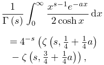
►
25.11.31
, .
…
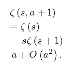
►
25.11.41
…
20: 1.8 Fourier Series
…
►where is square-integrable on and are given by (1.8.2), (1.8.4).
If is also square-integrable with Fourier coefficients or then
…
►Let be an absolutely integrable function of period , and continuous except at a finite number of points in any bounded interval.
…
►
