central in imaginary direction

(0.005 seconds)

1—10 of 945 matching pages

1: Mourad E. H. Ismail

… … ► 1944, in Cairo, Egypt) is a Distinguished Research Professor in the Department of Mathematics of the University of Central Florida. … ►His well-known book Classical and Quantum Orthogonal Polynomials in One Variable was published by Cambridge University Press in 2005 and reprinted with corrections in paperback in Ismail (2009). … ► 254, American Mathematical Society, 2000; Special Functions—Proceedings of the International Workshop, Hong Kong, June 21–25, 1999, World Scientific, 2000; Special Functions 2000: Current Perspective and Future Directions (with J. … Koelink), Developments in Mathematics, v. …

2: 18.1 Notation

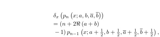
… ►Central differences in imaginary direction: … ►The main functions treated in this chapter are: … ►

Associated OP’s are denoted via addition of the letter $c$ at the end of the listing of parameters in their usual notations.

… ►

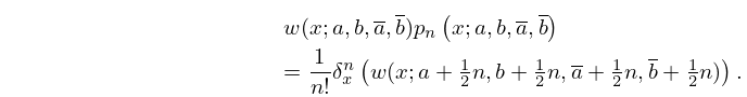
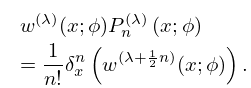
Classical OP’s in Two Variables

… ►In Koekoek et al. (2010)

\delta_{x}

denotes the operator

\mathrm{i}\delta_{x}

3: Gergő Nemes

… ► 1988 in Szeged, Hungary) is a Research Fellow at the Alfréd Rényi Institute of Mathematics in Budapest, Hungary. … ► in mathematics (with distinction) and a M. …in mathematics (with honours) from Loránd Eötvös University, Budapest, Hungary and a Ph. … in mathematics from Central European University in Budapest, Hungary. ►Nemes has research interests in asymptotic analysis, Écalle theory, exact WKB analysis, and special functions. …

4: 18.40 Methods of Computation

… ► … ►A simple set of choices is spelled out in Gordon (1968) which gives a numerically stable algorithm for direct computation of the recursion coefficients in terms of the moments, followed by construction of the J-matrix and quadrature weights and abscissas, and we will follow this approach: Let

N

be a positive integer and define … ►in which …The question is then: how is this possible given only

F_{N}(z)

, rather than

F(z)

itself?

F_{N}(z)

often converges to smooth results for

z

off the real axis for

\Im{z}

at a distance greater than the pole spacing of the

x_{n}

, this may then be followed by approximate numerical analytic continuation via fitting to lower order continued fractions (either Padé, see §3.11(iv), or pointwise continued fraction approximants, see Schlessinger (1968, Appendix)), to

F_{N}(z)

and evaluating these on the real axis in regions of higher pole density that those of the approximating function. … ►The quadrature points and weights can be put to a more direct and efficient use. …

5: 18.20 Hahn Class: Explicit Representations

… ►For comments on the use of the forward-difference operator

\Delta_{x}

, the backward-difference operator

\nabla_{x}

, and the central-difference operator

\delta_{x}

, see §18.2(ii). … ►In (18.20.1)

X

and

w_{x}

are as in Table 18.19.1. …For the Krawtchouk, Meixner, and Charlier polynomials,

F(x)

and

\kappa_{n}

are as in Table 18.20.1. … ►

18.20.3

w(x;a,b,\overline{a},\overline{b})p_{n}\left(x;a,b,\overline{a},\overline{b}% \right)=\frac{1}{n!}\delta_{x}^{n}\left(w(x;a+\tfrac{1}{2}n,b+\tfrac{1}{2}n,% \overline{a}+\tfrac{1}{2}n,\overline{b}+\tfrac{1}{2}n)\right).

ⓘ

Symbols:: $\delta_{\NVar{x}}$ : central difference, $\overline{\NVar{z}}$ : complex conjugate, $p_{\NVar{n}}\left(\NVar{x};\NVar{a},\NVar{b},\NVar{\overline{a}},\NVar{% \overline{b}}\right)$ : continuous Hahn polynomial, $!$ : factorial (as in $n!$ ), $n$ : nonnegative integer and $x$ : real variable
Referenced by:: §18.20(i)
Permalink:: http://dlmf.nist.gov/18.20.E3
Encodings:: pMML, png, TeX
See also:: Annotations for §18.20(i), §18.20(i), §18.20 and Ch.18

… ►

18.20.4

w^{(\lambda)}(x;\phi)P^{(\lambda)}_{n}\left(x;\phi\right)=\frac{1}{n!}\delta_{% x}^{n}\left(w^{(\lambda+\frac{1}{2}n)}(x;\phi)\right).

ⓘ

Symbols:: $P^{(\NVar{\lambda})}_{\NVar{n}}\left(\NVar{x};\NVar{\phi}\right)$ : Meixner–Pollaczek polynomial, $\delta_{\NVar{x}}$ : central difference, $!$ : factorial (as in $n!$ ), $n$ : nonnegative integer and $x$ : real variable
Referenced by:: §18.20(i)
Permalink:: http://dlmf.nist.gov/18.20.E4
Encodings:: pMML, png, TeX
See also:: Annotations for §18.20(i), §18.20(i), §18.20 and Ch.18

…

6: 18.22 Hahn Class: Recurrence Relations and Differences

… ►

§18.22(i) Recurrence Relations in $n$

… ►These polynomials satisfy (18.22.2) with

p_{n}(x)

A_{n}

, and

C_{n}

as in Table 18.22.1. … ►

§18.22(ii) Difference Equations in $x$

… ►For

A(x)

C(x)

, and

\lambda_{n}

in (18.22.12) see Table 18.22.2. … ►

18.22.27

\delta_{x}\left(p_{n}\left(x;a,b,\overline{a},\overline{b}\right)\right)=(n+2% \Re\left(a+b\right)-1)\*p_{n-1}\left(x;a+\tfrac{1}{2},b+\tfrac{1}{2},\overline% {a}+\tfrac{1}{2},\overline{b}+\tfrac{1}{2}\right),

ⓘ

Symbols:: $\delta_{\NVar{x}}$ : central difference, $\overline{\NVar{z}}$ : complex conjugate, $p_{\NVar{n}}\left(\NVar{x};\NVar{a},\NVar{b},\NVar{\overline{a}},\NVar{% \overline{b}}\right)$ : continuous Hahn polynomial, $\Re$ : real part, $n$ : nonnegative integer and $x$ : real variable
Referenced by:: §18.22(iii)
Permalink:: http://dlmf.nist.gov/18.22.E27
Encodings:: pMML, png, TeX
See also:: Annotations for §18.22(iii), §18.22(iii), §18.22 and Ch.18

…

7: 18.26 Wilson Class: Continued

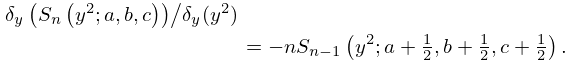
… ►For comments on the use of the forward-difference operator

\Delta_{x}

, the backward-difference operator

\nabla_{x}

, and the central-difference operator

\delta_{x}

, see §18.2(ii). … ►

18.26.14

\ifrac{\delta_{y}\left(W_{n}\left(y^{2};a,b,c,d\right)\right)}{\delta_{y}(y^{2% })}=-n(n+a+b+c+d-1)\*W_{n-1}\left(y^{2};a+\tfrac{1}{2},b+\tfrac{1}{2},c+\tfrac% {1}{2},d+\tfrac{1}{2}\right).

ⓘ

Symbols:: $W_{\NVar{n}}\left(\NVar{x};\NVar{a},\NVar{b},\NVar{c},\NVar{d}\right)$ : Wilson polynomial, $\delta_{\NVar{x}}$ : central difference, $y$ : real variable and $n$ : nonnegative integer
Referenced by:: §16.4(iii), §18.26(iii)
Permalink:: http://dlmf.nist.gov/18.26.E14
Encodings:: pMML, png, TeX
See also:: Annotations for §18.26(iii), §18.26 and Ch.18

►

18.26.15

\ifrac{\delta_{y}\left(S_{n}\left(y^{2};a,b,c\right)\right)}{\delta_{y}(y^{2})% }=-nS_{n-1}\left(y^{2};a+\tfrac{1}{2},b+\tfrac{1}{2},c+\tfrac{1}{2}\right).

ⓘ

Symbols:: $\delta_{\NVar{x}}$ : central difference, $S_{\NVar{n}}\left(\NVar{x};\NVar{a},\NVar{b},\NVar{c}\right)$ : continuous dual Hahn polynomial, $y$ : real variable and $n$ : nonnegative integer
Permalink:: http://dlmf.nist.gov/18.26.E15
Encodings:: pMML, png, TeX
See also:: Annotations for §18.26(iii), §18.26 and Ch.18

… ►Koornwinder (2009) rescales and reparametrizes Racah polynomials and Wilson polynomials in such a way that they are continuous in their four parameters, provided that these parameters are nonnegative. Moreover, if one or more of the new parameters becomes zero, then the polynomial descends to a lower family in the Askey scheme.

8: 10.73 Physical Applications

… ►Laplace’s equation governs problems in heat conduction, in the distribution of potential in an electrostatic field, and in hydrodynamics in the irrotational motion of an incompressible fluid. … ►This equation governs problems in acoustic and electromagnetic wave propagation. …Consequently, Bessel functions

J_{n}\left(x\right)

, and modified Bessel functions

I_{n}\left(x\right)

, are central to the analysis of microwave and optical transmission in waveguides, including coaxial and fiber. … ►More recently, Bessel functions appear in the inverse problem in wave propagation, with applications in medicine, astronomy, and acoustic imaging. … ►In quantum mechanics the spherical Bessel functions arise in the solution of the Schrödinger wave equation for a particle in a central potential. …

9: 18.19 Hahn Class: Definitions

… ►These eight further families can be grouped in two classes of OP’s: ►

Hahn class (or linear lattice class). These are OP’s $p_{n}(x)$ where the role of $\frac{\mathrm{d}}{\mathrm{d}x}$ is played by $\Delta_{x}$ or $\nabla_{x}$ or $\delta_{x}$ (see §18.1(i) for the definition of these operators). The Hahn class consists of four discrete and two continuous families.

►

Wilson class (or quadratic lattice class). These are OP’s $p_{n}(x)=p_{n}(\lambda(y))$ ( $p_{n}(x)$ of degree $n$ in $x$ , $\lambda(y)$ quadratic in $y$ ) where the role of the differentiation operator is played by $\tfrac{\Delta_{y}}{\Delta_{y}(\lambda(y))}$ or $\tfrac{\nabla_{y}}{\nabla_{y}(\lambda(y))}$ or $\tfrac{\delta_{y}}{\delta_{y}(\lambda(y))}$ . The Wilson class consists of two discrete and two continuous families.

►In addition to the limit relations in §18.7(iii) there are limit relations involving the further families in the Askey scheme, see §§18.21(ii) and 18.26(ii). The Askey scheme, depicted in Figure 18.21.1, gives a graphical representation of these limits. …

10: 36.15 Methods of Computation

… ►Close to the origin

\mathbf{x}=\boldsymbol{{0}}

of parameter space, the series in §36.8 can be used. … ►Far from the bifurcation set, the leading-order asymptotic formulas of §36.11 reproduce accurately the form of the function, including the geometry of the zeros described in §36.7. … ►Direct numerical evaluation can be carried out along a contour that runs along the segment of the real

t

-axis containing all real critical points of

\Phi

and is deformed outside this range so as to reach infinity along the asymptotic valleys of

\exp\left(i\Phi\right)

. …There is considerable freedom in the choice of deformations. … ►This can be carried out by direct numerical evaluation of canonical integrals along a finite segment of the real axis including all real critical points of

\Phi

, with contributions from the contour outside this range approximated by the first terms of an asymptotic series associated with the endpoints. …