central differences in imaginary direction

(0.006 seconds)

1—10 of 949 matching pages

1: 18.1 Notation

… ►

$x$ -Differences

►Forward differences: … ►Backward differences: … ►Central differences in imaginary direction: … ►In Koekoek et al. (2010)

\delta_{x}

denotes the operator

\mathrm{i}\delta_{x}

… … ► 1944, in Cairo, Egypt) is a Distinguished Research Professor in the Department of Mathematics of the University of Central Florida. … ►His well-known book Classical and Quantum Orthogonal Polynomials in One Variable was published by Cambridge University Press in 2005 and reprinted with corrections in paperback in Ismail (2009). … ► 254, American Mathematical Society, 2000; Special Functions—Proceedings of the International Workshop, Hong Kong, June 21–25, 1999, World Scientific, 2000; Special Functions 2000: Current Perspective and Future Directions (with J. … Koelink), Developments in Mathematics, v. …

3: Gergő Nemes

… ► 1988 in Szeged, Hungary) is a Research Fellow at the Alfréd Rényi Institute of Mathematics in Budapest, Hungary. … ► in mathematics (with distinction) and a M. …in mathematics (with honours) from Loránd Eötvös University, Budapest, Hungary and a Ph. … in mathematics from Central European University in Budapest, Hungary. ►Nemes has research interests in asymptotic analysis, Écalle theory, exact WKB analysis, and special functions. …

4: 18.22 Hahn Class: Recurrence Relations and Differences

§18.22 Hahn Class: Recurrence Relations and Differences

►

§18.22(i) Recurrence Relations in $n$

… ►These polynomials satisfy (18.22.2) with

p_{n}(x)

A_{n}

, and

C_{n}

as in Table 18.22.1. … ►

§18.22(ii) Difference Equations in $x$

… ►

§18.22(iii) $x$ -Differences

…

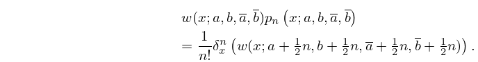
5: 18.20 Hahn Class: Explicit Representations

… ►For comments on the use of the forward-difference operator

\Delta_{x}

, the backward-difference operator

\nabla_{x}

, and the central-difference operator

\delta_{x}

, see §18.2(ii). … ►In (18.20.1)

X

and

w_{x}

are as in Table 18.19.1. …For the Krawtchouk, Meixner, and Charlier polynomials,

F(x)

and

\kappa_{n}

are as in Table 18.20.1. … ►

18.20.3

w(x;a,b,\overline{a},\overline{b})p_{n}\left(x;a,b,\overline{a},\overline{b}% \right)=\frac{1}{n!}\delta_{x}^{n}\left(w(x;a+\tfrac{1}{2}n,b+\tfrac{1}{2}n,% \overline{a}+\tfrac{1}{2}n,\overline{b}+\tfrac{1}{2}n)\right).

ⓘ

Symbols:: $\delta_{\NVar{x}}$ : central difference, $\overline{\NVar{z}}$ : complex conjugate, $p_{\NVar{n}}\left(\NVar{x};\NVar{a},\NVar{b},\NVar{\overline{a}},\NVar{% \overline{b}}\right)$ : continuous Hahn polynomial, $!$ : factorial (as in $n!$ ), $n$ : nonnegative integer and $x$ : real variable
Referenced by:: §18.20(i)
Permalink:: http://dlmf.nist.gov/18.20.E3
Encodings:: pMML, png, TeX
See also:: Annotations for §18.20(i), §18.20(i), §18.20 and Ch.18

… ►

18.20.4

w^{(\lambda)}(x;\phi)P^{(\lambda)}_{n}\left(x;\phi\right)=\frac{1}{n!}\delta_{% x}^{n}\left(w^{(\lambda+\frac{1}{2}n)}(x;\phi)\right).

ⓘ

Symbols:: $P^{(\NVar{\lambda})}_{\NVar{n}}\left(\NVar{x};\NVar{\phi}\right)$ : Meixner–Pollaczek polynomial, $\delta_{\NVar{x}}$ : central difference, $!$ : factorial (as in $n!$ ), $n$ : nonnegative integer and $x$ : real variable
Referenced by:: §18.20(i)
Permalink:: http://dlmf.nist.gov/18.20.E4
Encodings:: pMML, png, TeX
See also:: Annotations for §18.20(i), §18.20(i), §18.20 and Ch.18

…

6: 18.26 Wilson Class: Continued

… ►

§18.26(iii) Difference Relations

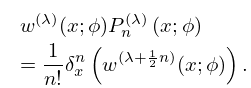
►For comments on the use of the forward-difference operator

\Delta_{x}

, the backward-difference operator

\nabla_{x}

, and the central-difference operator

\delta_{x}

, see §18.2(ii). ►For each family only the

y

-difference that lowers

n

is given. … ►Koornwinder (2009) rescales and reparametrizes Racah polynomials and Wilson polynomials in such a way that they are continuous in their four parameters, provided that these parameters are nonnegative. Moreover, if one or more of the new parameters becomes zero, then the polynomial descends to a lower family in the Askey scheme.

7: 18.40 Methods of Computation

… ►Usually, however, other methods are more efficient, especially the numerical solution of difference equations (§3.6) and the application of uniform asymptotic expansions (when available) for OP’s of large degree. … ►A simple set of choices is spelled out in Gordon (1968) which gives a numerically stable algorithm for direct computation of the recursion coefficients in terms of the moments, followed by construction of the J-matrix and quadrature weights and abscissas, and we will follow this approach: Let

N

be a positive integer and define … ►in which …The question is then: how is this possible given only

F_{N}(z)

, rather than

F(z)

itself?

F_{N}(z)

often converges to smooth results for

z

off the real axis for

\Im{z}

at a distance greater than the pole spacing of the

x_{n}

, this may then be followed by approximate numerical analytic continuation via fitting to lower order continued fractions (either Padé, see §3.11(iv), or pointwise continued fraction approximants, see Schlessinger (1968, Appendix)), to

F_{N}(z)

and evaluating these on the real axis in regions of higher pole density that those of the approximating function. … ►The quadrature points and weights can be put to a more direct and efficient use. …

8: 18.19 Hahn Class: Definitions

… ►The Askey scheme extends the three families of classical OP’s (Jacobi, Laguerre and Hermite) with eight further families of OP’s for which the role of the differentiation operator

\frac{\mathrm{d}}{\mathrm{d}x}

in the case of the classical OP’s is played by a suitable difference operator. These eight further families can be grouped in two classes of OP’s: ►

Hahn class (or linear lattice class). These are OP’s $p_{n}(x)$ where the role of $\frac{\mathrm{d}}{\mathrm{d}x}$ is played by $\Delta_{x}$ or $\nabla_{x}$ or $\delta_{x}$ (see §18.1(i) for the definition of these operators). The Hahn class consists of four discrete and two continuous families.

►

Wilson class (or quadratic lattice class). These are OP’s $p_{n}(x)=p_{n}(\lambda(y))$ ( $p_{n}(x)$ of degree $n$ in $x$ , $\lambda(y)$ quadratic in $y$ ) where the role of the differentiation operator is played by $\tfrac{\Delta_{y}}{\Delta_{y}(\lambda(y))}$ or $\tfrac{\nabla_{y}}{\nabla_{y}(\lambda(y))}$ or $\tfrac{\delta_{y}}{\delta_{y}(\lambda(y))}$ . The Wilson class consists of two discrete and two continuous families.

►In addition to the limit relations in §18.7(iii) there are limit relations involving the further families in the Askey scheme, see §§18.21(ii) and 18.26(ii). …

9: 16.25 Methods of Computation

… ►They are similar to those described for confluent hypergeometric functions, and hypergeometric functions in §§13.29 and 15.19. There is, however, an added feature in the numerical solution of differential equations and difference equations (recurrence relations). This occurs when the wanted solution is intermediate in asymptotic growth compared with other solutions. In these cases integration, or recurrence, in either a forward or a backward direction is unstable. …

10: Sidebar 9.SB1: Supernumerary Rainbows

… ►The faint line below the main colored arc is a ‘supernumerary rainbow’, produced by the interference of different sun-rays traversing a raindrop and emerging in the same direction. …Airy invented his function in 1838 precisely to describe this phenomenon more accurately than Young had done in 1800 when pointing out that supernumerary rainbows require the wave theory of light and are impossible to explain with Newton’s picture of light as a stream of independent corpuscles. The house in the picture is Newton’s birthplace. …