case%20%CE%BB%3D0

SearchAdvancedHelp

(0.004 seconds)

1—10 of 664 matching pages

1: 34.2 Definition: $\mathit{3}j$ Symbol

§34.2 Definition: $\mathit{3}j$ Symbol

►The quantities $j_1,j_2,j_3$ in the $\mathit{3}j$ symbol are called angular momenta. …They therefore satisfy the triangle conditions …where $r,s,t$ is any permutation of $1,2,3$. The corresponding projective quantum numbers $m_1,m_2,m_3$ are given by …

2: 28.35 Tables

… ►

Blanch and Clemm (1965) includes values of ${\mathrm{Mc}}_n^{(2)}(x,\sqrt{q})$, $\mathrm{Mc}_n^{(2)}{}_{}{}^{\prime }(x,\sqrt{q})$ for $n=0(1)7$, $x=0(.02)1$; $n=8(1)15$, $x=0(.01)1$. Also ${\mathrm{Ms}}_n^{(2)}(x,\sqrt{q})$, $\mathrm{Ms}_n^{(2)}{}_{}{}^{\prime }(x,\sqrt{q})$ for $n=1(1)7$, $x=0(.02)1$; $n=8(1)15$, $x=0(.01)1$. In all cases $q=0(.05)1$. Precision is generally 7D. Approximate formulas and graphs are also included.

… ►

Ince (1932) includes eigenvalues $a_n$, $b_n$, and Fourier coefficients for $n=0$ or $1(1)6$, $q=0(1)10(2)20(4)40$; 7D. Also ${\mathrm{ce}}_n(x,q)$, ${\mathrm{se}}_n(x,q)$ for $q=0(1)10$, $x=1(1)90$, corresponding to the eigenvalues in the tables; 5D. Notation: $a_n={\mathrm{𝑏𝑒}}_n-2q$, $b_n={\mathrm{𝑏𝑜}}_n-2q$.

►

Kirkpatrick (1960) contains tables of the modified functions ${\mathrm{Ce}}_n(x,q)$, ${\mathrm{Se}}_{n+1}(x,q)$ for $n=0(1)5$, $q=1(1)20$, $x=0.1(.1)1$; 4D or 5D.

►

National Bureau of Standards (1967) includes the eigenvalues $a_n\left(q\right)$, $b_n\left(q\right)$ for $n=0(1)3$ with $q=0(.2)20(.5)37(1)100$, and $n=4(1)15$ with $q=0(2)100$; Fourier coefficients for ${\mathrm{ce}}_n(x,q)$ and ${\mathrm{se}}_n(x,q)$ for $n=0(1)15$, $n=1(1)15$, respectively, and various values of $q$ in the interval $[0,100]$; joining factors $g_{e,n}(\sqrt{q})$, $f_{e,n}(\sqrt{q})$ for $n=0(1)15$ with $q=0(.5\text{ to }10)100$ (but in a different notation). Also, eigenvalues for large values of $q$. Precision is generally 8D.

… ►

Zhang and Jin (1996, pp. 521–532) includes the eigenvalues $a_n\left(q\right)$, $b_{n+1}\left(q\right)$ for $n=0(1)4$, $q=0(1)50$; $n=0(1)20$ ($a$’s) or 19 ($b$’s), $q=1,3,5,10,15,25,50(50)200$. Fourier coefficients for ${\mathrm{ce}}_n(x,10)$, ${\mathrm{se}}_{n+1}(x,10)$, $n=0(1)7$. Mathieu functions ${\mathrm{ce}}_n(x,10)$, ${\mathrm{se}}_{n+1}(x,10)$, and their first $x$-derivatives for $n=0(1)4$, $x=0(5^{\circ }){90}^{\circ }$. Modified Mathieu functions ${\mathrm{Mc}}_n^{(j)}(x,\sqrt{10})$, ${\mathrm{Ms}}_{n+1}^{(j)}(x,\sqrt{10})$, and their first $x$-derivatives for $n=0(1)4$, $j=1,2$, $x=0(.2)4$. Precision is mostly 9S.

…

3: 23.23 Tables

… ►2 in Abramowitz and Stegun (1964) gives values of $\mathrm{\wp }\left(z\right)$, ${\mathrm{\wp }}^{\prime }\left(z\right)$, and $\zeta \left(z\right)$ to 7 or 8D in the rectangular and rhombic cases, normalized so that ${\omega }_1=1$ and ${\omega }_3=\mathrm{i}a$ (rectangular case), or ${\omega }_1=1$ and ${\omega }_3=\frac{1}{2}+\mathrm{i}a$ (rhombic case), for $a$ = 1. …05, and in the case of $\mathrm{\wp }\left(z\right)$ the user may deduce values for complex $z$ by application of the addition theorem (23.10.1). ►Abramowitz and Stegun (1964) also includes other tables to assist the computation of the Weierstrass functions, for example, the generators as functions of the lattice invariants $g_2$ and $g_3$. …

4: 23.4 Graphics

… ►

§23.4(i) Real Variables

►Line graphs of the Weierstrass functions $\mathrm{\wp }\left(x\right)$, $\zeta \left(x\right)$, and $\sigma \left(x\right)$, illustrating the lemniscatic and equianharmonic cases. … ►

►►

Figure 23.4.1: $\mathrm{\wp }(x;g_2,0)$ for $0\le x\le 9$, $g_2$ = 0. …(Lemniscatic case.) Magnify

►

►►

Figure 23.4.2: $\mathrm{\wp }(x;0,g_3)$ for $0\le x\le 9$, $g_3$ = 0. …(Equianharmonic case.) Magnify

►

►►

Figure 23.4.3: $\zeta (x;g_2,0)$ for $0\le x\le 8$, $g_2$ = 0. …(Lemniscatic case.) Magnify

…

5: 23.5 Special Lattices

… ►In this case the lattice roots $e_1$, $e_2$, and $e_3$ are real and distinct. … ► $e_1$ and $g_3$ have the same sign unless $2{\omega }_3=(1+\mathrm{i}){\omega }_1$ when both are zero: the pseudo-lemniscatic case. As a function of $\mathrm{\Im }{e}_3$ the root $e_1$ is increasing. For the case ${\omega }_3={\mathrm{e}}^{\pi \mathrm{i}/3}{\omega }_1$ see §23.5(v). … ►Note also that in this case $\tau ={\mathrm{e}}^{\mathrm{i}\pi /3}$. …

6: 28.1 Special Notation

… ► ►►

${\mathrm{Ce}}_{\nu }(z,q)$,	${\mathrm{Se}}_{\nu }(z,q)$,	${\mathrm{Fe}}_n(z,q)$,	${\mathrm{Ge}}_n(z,q)$,
…

… ►

$${\mathrm{Me}}_n^{(1,2)}(z,q)=\sqrt{\frac{1}{2}\pi }{g}_{e,n}(h){\mathrm{ce}}_n(0,q){\mathrm{Mc}}_n^{(3,4)}(z,h),$$

… ►

$${\mathrm{Ne}}_n^{(1,2)}(z,q)=\sqrt{\frac{1}{2}\pi }{g}_{o,n}(h){\mathrm{se}}_n^{\prime }(0,q){\mathrm{Ms}}_n^{(3,4)}(z,h).$$

… ►

${\mathrm{in}}_n={\mathrm{fe}}_n,$ ${\mathrm{ceh}}_n={\mathrm{Ce}}_n,$ ${\mathrm{inh}}_n={\mathrm{Fe}}_n,$

… ►

Abramowitz and Stegun (1964, Chapter 20)

…

7: 32.8 Rational Solutions

… ►The rational solutions when the parameters satisfy (32.8.22) are special cases of §32.10(iv). … ►Cases (a) and (b) are special cases of §32.10(v). … ►For the case $\delta =0$ see Airault (1979) and Lukaševič (1968). … ►In the general case, ${\text{P}}_{\text{VI}}$ has rational solutions if …These are special cases of §32.10(vi). …

8: 25.12 Polylogarithms

… ►

25.12.5 $${\mathrm{Li}}_2\left(z^m\right)=m\sum _{k=0}^{m-1}{\mathrm{Li}}_2\left(z{\mathrm{e}}^{2\pi \mathrm{i}k/m}\right),$$ $m=1,2,3,\mathrm{\dots }$, .

ⓘ

Symbols:

$\pi$: the ratio of the circumference of a circle to its diameter, ${\mathrm{Li}}_2\left(z\right)$: dilogarithm, $\mathrm{e}$: base of natural logarithm, $\mathrm{i}$: imaginary unit, $k$: nonnegative integer, $m$: nonnegative integer and $z$: complex variable

Source:

Maximon (2003, (3.12), p. 2809)

Permalink:

http://dlmf.nist.gov/25.12.E5

Encodings:

pMML, png, TeX

See also:

Annotations for §25.12(i), §25.12 and Ch.25

… ►

►►

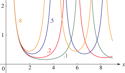
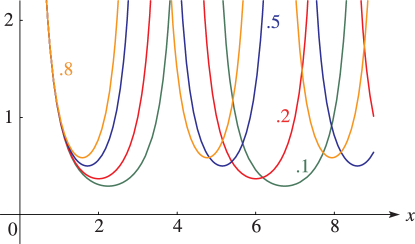
Figure 25.12.1: Dilogarithm function ${\mathrm{Li}}_2\left(x\right)$, Magnify

►

►

►

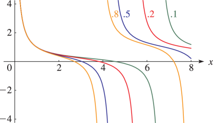
Figure 25.12.2: Absolute value of the dilogarithm function $\left|{\mathrm{Li}}_2\left(x+\mathrm{i}y\right)\right|$, $-20\le x\le 20$, $-20\le y\le 20$. … Magnify 3D Help

… ►The special case $z=1$ is the Riemann zeta function: $\zeta \left(s\right)={\mathrm{Li}}_s\left(1\right)$. … ►(In the latter case (25.12.11) becomes (25.5.1)). …

9: 27.2 Functions

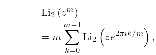
… ►Euclid’s Elements (Euclid (1908, Book IX, Proposition 20)) gives an elegant proof that there are infinitely many primes. … ►It is the special case $k=2$ of the function $d_k\left(n\right)$ that counts the number of ways of expressing $n$ as the product of $k$ factors, with the order of factors taken into account. … ►

Table 27.2.2: Functions related to division.

► ►►►►►

$n$	$\varphi \left(n\right)$	$d\left(n\right)$	$\sigma \left(n\right)$	$n$	$\varphi \left(n\right)$	$d\left(n\right)$	$\sigma \left(n\right)$	$n$	$\varphi \left(n\right)$	$d\left(n\right)$	$\sigma \left(n\right)$	$n$	$\varphi \left(n\right)$	$d\left(n\right)$	$\sigma \left(n\right)$
…
5	4	2	6	18	6	6	39	31	30	2	32	44	20	6	84
…
7	6	2	8	20	8	6	42	33	20	4	48	46	22	4	72
…
12	4	6	28	25	20	3	31	38	18	4	60	51	32	4	72
…

►

10: Guide to Searching the DLMF

… ►All terms are taken to be case-insensitive, except those taken to represent math expressions (see Case Sensitivity). … ►Note that the first form may match other functions $K$ than the Bessel $K$ function, so if you are sure you want Bessel $K$, you might as well enter one of the other 3 forms. ►

Case Sensitivity

►DLMF search is generally case-insensitive except when it is important to be case-sensitive, as when two different special functions have the same standard names but one name has a lower-case initial and the other is has an upper-case initial, such as si and Si, gamma and Gamma. In the following situations, DLMF search is case-sensitive: …