by%20parts

SearchAdvancedHelp

(0.002 seconds)

1—10 of 37 matching pages

1: 28 Mathieu Functions and Hill’s Equation

…

2: 22.3 Graphics

… ►

►►

Figure 22.3.26: Density plot of $|\mathrm{sn}(5,k)|$ as a function of complex $k^2$, $-10\le \mathrm{\Re }\left(k^2\right)\le 20$, $-10\le \mathrm{\Im }\left(k^2\right)\le 10$. … Magnify

►

►►

Figure 22.3.27: Density plot of $|\mathrm{sn}(10,k)|$ as a function of complex $k^2$, $-10\le \mathrm{\Re }\left(k^2\right)\le 20$, $-10\le \mathrm{\Im }\left(k^2\right)\le 10$. … Magnify

►

►►

Figure 22.3.28: Density plot of $|\mathrm{sn}(20,k)|$ as a function of complex $k^2$, $-10\le \mathrm{\Re }\left(k^2\right)\le 20$, $-10\le \mathrm{\Im }\left(k^2\right)\le 10$. … Magnify

►

►►

Figure 22.3.29: Density plot of $|\mathrm{sn}(30,k)|$ as a function of complex $k^2$, $-10\le \mathrm{\Re }\left(k^2\right)\le 20$, $-10\le \mathrm{\Im }\left(k^2\right)\le 10$. … Magnify

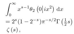
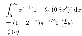
3: 20.10 Integrals

… ►

20.10.1 $${\int }_0^{\mathrm{\infty }}{x}^{s-1}{\theta }_2\left(0\right|\mathrm{i}{x}^2)dx=2^s(1-2^{-s}){\pi }^{-s/2}\mathrm{\Gamma }\left(\frac{1}{2}s\right)\zeta \left(s\right),$$ $\mathrm{\Re }s>1$,

ⓘ

Symbols:

$\mathrm{\Gamma }\left(z\right)$: gamma function, ${\theta }_j\left(z\right|\tau )$: theta function, $\zeta \left(s\right)$: Riemann zeta function, $\pi$: the ratio of the circumference of a circle to its diameter, $dx$: differential of $x$ , $\mathrm{i}$: imaginary unit, $\int$: integral and $\mathrm{\Re }$: real part

Keywords:

Mellin transform

Referenced by:

§20.10(i), Erratum (V1.1.5) for §20.10(i)

Permalink:

http://dlmf.nist.gov/20.10.E1

Encodings:

pMML, png, TeX

Modification (effective with 1.1.5):

Originally the constraint was $\mathrm{\Re }s>2$. This can be relaxed to $\mathrm{\Re }s>1$ because ${\theta }_2\left(0\right|\mathrm{i}{x}^2)=x^{-1}{\theta }_4\left(0\right|\mathrm{i}{x}^{-2})\sim x^{-1}$ as $x\to 0+$, which follows from (20.7.31) and (20.4.5).

See also:

Annotations for §20.10(i), §20.10 and Ch.20

►

20.10.2 $${\int }_0^{\mathrm{\infty }}{x}^{s-1}({\theta }_3\left(0\right|\mathrm{i}{x}^2)-1)dx={\pi }^{-s/2}\mathrm{\Gamma }\left(\frac{1}{2}s\right)\zeta \left(s\right),$$ $\mathrm{\Re }s>1$,

ⓘ

Symbols:

$\mathrm{\Gamma }\left(z\right)$: gamma function, ${\theta }_j\left(z\right|\tau )$: theta function, $\zeta \left(s\right)$: Riemann zeta function, $\pi$: the ratio of the circumference of a circle to its diameter, $dx$: differential of $x$ , $\mathrm{i}$: imaginary unit, $\int$: integral and $\mathrm{\Re }$: real part

Keywords:

Mellin transform

Referenced by:

§20.10(i), Erratum (V1.1.5) for §20.10(i)

Permalink:

http://dlmf.nist.gov/20.10.E2

Encodings:

pMML, png, TeX

Modification (effective with 1.1.5):

Originally the constraint was $\mathrm{\Re }s>2$. This can be relaxed to $\mathrm{\Re }s>1$ because ${\theta }_3\left(0\right|\mathrm{i}{x}^2)=x^{-1}{\theta }_3\left(0\right|\mathrm{i}{x}^{-2})\sim x^{-1}$ as $x\to 0+$, which follows from (20.7.32) and (20.4.4).

See also:

Annotations for §20.10(i), §20.10 and Ch.20

►

20.10.3 $${\int }_0^{\mathrm{\infty }}{x}^{s-1}(1-{\theta }_4\left(0\right|\mathrm{i}{x}^2))dx=(1-2^{1-s}){\pi }^{-s/2}\mathrm{\Gamma }\left(\frac{1}{2}s\right)\zeta \left(s\right),$$ $\mathrm{\Re }s>0$.

ⓘ

Symbols:

$\mathrm{\Gamma }\left(z\right)$: gamma function, ${\theta }_j\left(z\right|\tau )$: theta function, $\zeta \left(s\right)$: Riemann zeta function, $\pi$: the ratio of the circumference of a circle to its diameter, $dx$: differential of $x$ , $\mathrm{i}$: imaginary unit, $\int$: integral and $\mathrm{\Re }$: real part

Keywords:

Mellin transform

Referenced by:

§20.10(i), Erratum (V1.1.5) for §20.10(i)

Permalink:

http://dlmf.nist.gov/20.10.E3

Encodings:

pMML, png, TeX

Modification (effective with 1.1.5):

Originally the constraint was $\mathrm{\Re }s>2$. This can be relaxed to $\mathrm{\Re }s>0$ because $1-{\theta }_4\left(0\right|\mathrm{i}{x}^2)=1-x^{-1}{\theta }_2\left(0\right|\mathrm{i}{x}^{-2})\sim 1$ as $x\to 0+$, which follows from (20.7.33) and (20.4.3).

See also:

Annotations for §20.10(i), §20.10 and Ch.20

… ►Let $s$, $\mathrm{\ell }$, and $\beta$ be constants such that $\mathrm{\Re }s>0$, $\mathrm{\ell }>0$, and $\left|\mathrm{\Re }\beta \right|+\left|\mathrm{\Im }\beta \right|\le \mathrm{\ell }$. …

4: 20 Theta Functions

Chapter 20 Theta Functions

…

5: 6.19 Tables

… ►

Abramowitz and Stegun (1964, Chapter 5) includes the real and imaginary parts of $z{\mathrm{e}}^z{E}_1\left(z\right)$, $x=-19(1)20$, $y=0(1)20$, 6D; ${\mathrm{e}}^z{E}_1\left(z\right)$, $x=-4(.5)-2$, $y=0(.2)1$, 6D; $E_1\left(z\right)+\ln z$, $x=-2(.5)2.5$, $y=0(.2)1$, 6D.

►

Zhang and Jin (1996, pp. 690–692) includes the real and imaginary parts of $E_1\left(z\right)$, $\pm x=0.5,1,3,5,10,15,20,50,100$, $y=0(.5)1(1)5(5)30,50,100$, 8S.

6: 9.18 Tables

… ►

Zhang and Jin (1996, p. 337) tabulates $\mathrm{Ai}\left(x\right)$, ${\mathrm{Ai}}^{\prime }\left(x\right)$, $\mathrm{Bi}\left(x\right)$, ${\mathrm{Bi}}^{\prime }\left(x\right)$ for $x=0(1)20$ to 8S and for $x=-20(1)0$ to 9D.

… ►

Woodward and Woodward (1946) tabulates the real and imaginary parts of $\mathrm{Ai}\left(z\right)$, ${\mathrm{Ai}}^{\prime }\left(z\right)$, $\mathrm{Bi}\left(z\right)$, ${\mathrm{Bi}}^{\prime }\left(z\right)$ for $\mathrm{\Re }z=-2.4(.2)2.4$, $\mathrm{\Im }z=-2.4(.2)0$. Precision is 4D.

… ►

Miller (1946) tabulates $a_k$, ${\mathrm{Ai}}^{\prime }\left(a_k\right)$, $a_k^{\prime }$, $\mathrm{Ai}\left(a_k^{\prime }\right)$, $k=1(1)50$; $b_k$, ${\mathrm{Bi}}^{\prime }\left(b_k\right)$, $b_k^{\prime }$, $\mathrm{Bi}\left(b_k^{\prime }\right)$, $k=1(1)20$. Precision is 8D. Entries for $k=1(1)20$ are reproduced in Abramowitz and Stegun (1964, Chapter 10).

►

Sherry (1959) tabulates $a_k$, ${\mathrm{Ai}}^{\prime }\left(a_k\right)$, $a_k^{\prime }$, $\mathrm{Ai}\left(a_k^{\prime }\right)$, $k=1(1)50$; 20S.

… ►

Corless et al. (1992) gives the real and imaginary parts of ${\beta }_k$ for $k=1(1)13$; 14S.

…

7: 8 Incomplete Gamma and Related
Functions

…

8: 23 Weierstrass Elliptic and Modular
Functions

…

9: 7.23 Tables

… ►

Zhang and Jin (1996, pp. 638, 640–641) includes the real and imaginary parts of $\mathrm{erf}z$, $x\in [0,5]$, $y=0.5(.5)3$, 7D and 8D, respectively; the real and imaginary parts of ${\int }_x^{\mathrm{\infty }}{\mathrm{e}}^{\pm \mathrm{i}{t}^2}dt$, $(1/\sqrt{\pi }){\mathrm{e}}^{\mp \mathrm{i}(x^2+(\pi /4))}{\int }_x^{\mathrm{\infty }}{\mathrm{e}}^{\pm \mathrm{i}{t}^2}dt$, $x=0(.5)20(1)25$, 8D, together with the corresponding modulus and phase to 8D and 6D (degrees), respectively.

…

10: 10.75 Tables

… ►

Zhang and Jin (1996, pp. 185–195) tabulates $J_n\left(x\right)$, $J_n^{\prime }\left(x\right)$, $Y_n\left(x\right)$, $Y_n^{\prime }\left(x\right)$, $n=0(1)10(10)50,100$, $x=1$, 5, 10, 25, 50, 100, 9S; $J_{n+\alpha }\left(x\right)$, $J_{n+\alpha }^{\prime }\left(x\right)$, $Y_{n+\alpha }\left(x\right)$, $Y_{n+\alpha }^{\prime }\left(x\right)$, $n=0(1)5,10,30,50,100$, $\alpha =\frac{1}{4},\frac{1}{3},\frac{1}{2},\frac{2}{3},\frac{3}{4}$, $x=1,5,10,50$, 8S; real and imaginary parts of $J_{n+\alpha }\left(z\right)$, $J_{n+\alpha }^{\prime }\left(z\right)$, $Y_{n+\alpha }\left(z\right)$, $Y_{n+\alpha }^{\prime }\left(z\right)$, $n=0(1)15,20(10)50,100$, $\alpha =0,\frac{1}{2}$, $z=4+2\mathrm{i}$, $20+10\mathrm{i}$, 8S.

… ►

Zhang and Jin (1996, pp. 240–250) tabulates $I_n\left(x\right)$, $I_n^{\prime }\left(x\right)$, $K_n\left(x\right)$, $K_n^{\prime }\left(x\right)$, $n=0(1)10(10)50,100$, $x=1,5,10,25,50,100$, 9S; $I_{n+\alpha }\left(x\right)$, $I_{n+\alpha }^{\prime }\left(x\right)$, $K_{n+\alpha }\left(x\right)$, $K_{n+\alpha }^{\prime }\left(x\right)$, $n=0(1)5$, 10, 30, 50, 100, $\alpha =\frac{1}{4}$, $\frac{1}{3}$, $\frac{1}{2}$, $\frac{2}{3}$, $\frac{3}{4}$, $x=1$, 5, 10, 50, 8S; real and imaginary parts of $I_{n+\alpha }\left(z\right)$, $I_{n+\alpha }^{\prime }\left(z\right)$, $K_{n+\alpha }\left(z\right)$, $K_{n+\alpha }^{\prime }\left(z\right)$, $n=0(1)15$, 20(10)50, 100, $\alpha =0,\frac{1}{2}$, $z=4+2\mathrm{i},20+10\mathrm{i}$, 8S.

… ►

Zhang and Jin (1996, pp. 296–305) tabulates ${𝗃}_n\left(x\right)$, ${𝗃}_n^{\prime }\left(x\right)$, ${𝗒}_n\left(x\right)$, ${𝗒}_n^{\prime }\left(x\right)$, ${𝗂}_n^{(1)}\left(x\right)$, $𝗂_n^{(1)}{}_{}{}^{\prime }\left(x\right)$, ${𝗄}_n\left(x\right)$, ${𝗄}_n^{\prime }\left(x\right)$, $n=0(1)10(10)30$, 50, 100, $x=1$, 5, 10, 25, 50, 100, 8S; $x{𝗃}_n\left(x\right)$, ${(x{𝗃}_n\left(x\right))}^{\prime }$, $x{𝗒}_n\left(x\right)$, ${(x{𝗒}_n\left(x\right))}^{\prime }$ (Riccati–Bessel functions and their derivatives), $n=0(1)10(10)30$, 50, 100, $x=1$, 5, 10, 25, 50, 100, 8S; real and imaginary parts of ${𝗃}_n\left(z\right)$, ${𝗃}_n^{\prime }\left(z\right)$, ${𝗒}_n\left(z\right)$, ${𝗒}_n^{\prime }\left(z\right)$, ${𝗂}_n^{(1)}\left(z\right)$, $𝗂_n^{(1)}{}_{}{}^{\prime }\left(z\right)$, ${𝗄}_n\left(z\right)$, ${𝗄}_n^{\prime }\left(z\right)$, $n=0(1)15$, 20(10)50, 100, $z=4+2\mathrm{i}$, $20+10\mathrm{i}$, 8S. (For the notation replace $j,y,\mathrm{i},k$ by $𝗃$, $𝗒$, ${𝗂}^{(1)}$, $𝗄$, respectively.)

…