behavior at singularities
(0.002 seconds)
1—10 of 12 matching pages
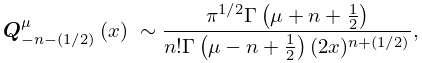
1: 14.8 Behavior at Singularities
2: 14.21 Definitions and Basic Properties
…
►
§14.21(iii) Properties
… ►This includes, for example, the Wronskian relations (14.2.7)–(14.2.11); hypergeometric representations (14.3.6)–(14.3.10) and (14.3.15)–(14.3.20); results for integer orders (14.6.3)–(14.6.5), (14.6.7), (14.6.8), (14.7.6), (14.7.7), and (14.7.11)–(14.7.16); behavior at singularities (14.8.7)–(14.8.16); connection formulas (14.9.11)–(14.9.16); recurrence relations (14.10.3)–(14.10.7). …3: 14.20 Conical (or Mehler) Functions
…
►
§14.20(iii) Behavior as
…4: 19.12 Asymptotic Approximations
…
►With denoting the digamma function (§5.2(i)) in this subsection, the asymptotic behavior of and near the singularity at
is given by the following convergent series:
…
5: 2.10 Sums and Sequences
…
►For extensions of the Euler–Maclaurin formula to functions with singularities at
or (or both) see Sidi (2004, 2012b, 2012a).
…
►We seek the behavior as .
…
►
(b´)
…
►The singularities of on the unit circle are branch points at
.
To match the limiting behavior of
at these points we set
…
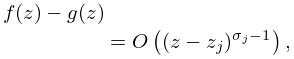
On the circle , the function has a finite number of singularities, and at each singularity , say,
2.10.30
,
where is a positive constant.
6: 8.12 Uniform Asymptotic Expansions for Large Parameter
…
►The right-hand sides of equations (8.12.9), (8.12.10) have removable singularities at
, and the Maclaurin series expansion of is given by
…
►For the asymptotic behavior of as see Dunster et al. (1998) and Olde Daalhuis (1998c).
…
►A different type of uniform expansion with coefficients that do not possess a removable singularity at
is given by
…
7: 2.7 Differential Equations
…
►All solutions are analytic at an ordinary point, and their Taylor-series expansions are found by equating coefficients.
…
►If both and are analytic at
, then is a regular singularity (or singularity of the first kind).
…
►The most common type of irregular singularity for special functions has rank 1 and is located at infinity.
…
►The transformed differential equation either has a regular singularity at
, or its characteristic equation has unequal roots.
…
►For irregular singularities of nonclassifiable rank, a powerful tool for finding the asymptotic behavior of solutions, complete with error bounds, is as follows:
…
8: 1.8 Fourier Series
…
►
Lebesgue Constants
… ►(1.8.10) continues to apply if either or or both are infinite and/or has finitely many singularities in , provided that the integral converges uniformly (§1.5(iv)) at , and the singularities for all sufficiently large . … ►Let be an absolutely integrable function of period , and continuous except at a finite number of points in any bounded interval. …at every point at which has both a left-hand derivative (that is, (1.4.4) applies when ) and a right-hand derivative (that is, (1.4.4) applies when ). The convergence is non-uniform, however, at points where ; see §6.16(i). …9: 1.18 Linear Second Order Differential Operators and Eigenfunction Expansions
…
►
…
►Note that the integral in (1.18.66) is not singular if approached separately from above, or below, the real axis: in fact analytic continuation from the upper half of the complex plane, across the cut, and onto higher Riemann Sheets can access complex poles with singularities at discrete energies corresponding to quantum resonances, or decaying quantum states with lifetimes proportional to .
For this latter see Simon (1973), and Reinhardt (1982); wherein advantage is taken of the fact that although branch points are actual singularities of an analytic function, the location of the branch cuts are often at our disposal, as they are not singularities of the function, but simply arbitrary lines to keep a function single valued, and thus only singularities of a specific representation of that analytic function.
…
►In unusual cases , even for all , such as in the case of the Schrödinger–Coulomb problem () discussed in §18.39 and §33.14, where the point spectrum actually accumulates at the onset of the continuum at
, implying an essential singularity, as well as a branch point, in matrix elements of the resolvent, (1.18.66).
…
►Similarly at
.
…
10: Bibliography B
…
►
Singularities in Waves and Rays.
In Les Houches Lecture Series Session XXXV, R. Balian, M. Kléman, and J.-P. Poirier (Eds.),
Vol. 35, pp. 453–543.
…
►
Uniform asymptotic expansions of integrals with stationary point near algebraic singularity.
Comm. Pure Appl. Math. 19, pp. 353–370.
►
Uniform asymptotic expansions of integrals with many nearby stationary points and algebraic singularities.
J. Math. Mech. 17, pp. 533–559.
…
►
Asymptotic behavior of the Pollaczek polynomials and their zeros.
Stud. Appl. Math. 96, pp. 307–338.
…
►
The behavior at unit argument of the hypergeometric function
.
SIAM J. Math. Anal. 18 (5), pp. 1227–1234.
…
