backward

SearchAdvancedHelp

(0.001 seconds)

1—10 of 21 matching pages

1: 5.21 Methods of Computation

… ►An effective way of computing $\mathrm{\Gamma }\left(z\right)$ in the right half-plane is backward recurrence, beginning with a value generated from the asymptotic expansion (5.11.3). …For the left half-plane we can continue the backward recurrence or make use of the reflection formula (5.5.3). …

2: 16.25 Methods of Computation

… ►In these cases integration, or recurrence, in either a forward or a backward direction is unstable. …

3: Browsers

… ►Although we have attempted to follow standards and maintain backwards compatibility with older browsers, you will generally get the best results by upgrading to the latest version of your preferred browser.

4: 11.13 Methods of Computation

… ►The solution ${𝐊}_{\nu }\left(x\right)$ needs to be integrated backwards for small $x$, and either forwards or backwards for large $x$ depending whether or not $\nu$ exceeds $\frac{1}{2}$. For ${𝐌}_{\nu }\left(x\right)$ both forward and backward integration are unstable, and boundary-value methods are required (§3.7(iii)). … ►In consequence forward recurrence, backward recurrence, or boundary-value methods may be necessary. …

5: 3.6 Linear Difference Equations

… ► … ►Because the recessive solution of a homogeneous equation is the fastest growing solution in the backward direction, it occurred to J. …A “trial solution” is then computed by backward recursion, in the course of which the original components of the unwanted solution $g_n$ die away. … ►Then $w_n$ is generated by backward recursion from … ►Thus in the inhomogeneous case it may sometimes be necessary to recur backwards to achieve stability. …

6: 18.1 Notation

… ►Backward differences: ►

$${\nabla }_x\left(f(x)\right)=f(x)-f(x-1),$$

►

$${\nabla }_x^{n+1}\left(f(x)\right)={\nabla }_x\left({\nabla }_x^n(f(x))\right).$$

…

7: 7.22 Methods of Computation

… ►See Gautschi (1977a), where forward and backward recursions are used; see also Gautschi (1961). …

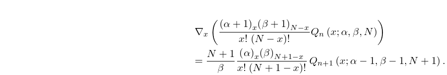
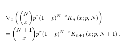
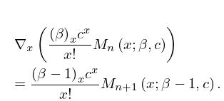
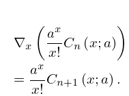
8: 18.22 Hahn Class: Recurrence Relations and Differences

… ►

18.22.20 $${\nabla }_x\left(\frac{{\left(\alpha +1\right)}_x{\left(\beta +1\right)}_{N-x}}{x!(N-x)!}{Q}_n(x;\alpha ,\beta ,N)\right)=\frac{N+1}{\beta }\frac{{\left(\alpha \right)}_x{\left(\beta \right)}_{N+1-x}}{x!(N+1-x)!}{Q}_{n+1}(x;\alpha -1,\beta -1,N+1).$$

ⓘ

Symbols:

$Q_n(x;\alpha ,\beta ,N)$: Hahn polynomial, ${\left(a\right)}_n$: Pochhammer’s symbol (or shifted factorial), ${\nabla }_x$: backward difference, $!$: factorial (as in $n!$), $N$: positive integer, $n$: nonnegative integer and $x$: real variable

Referenced by:

§16.4(iii)

Permalink:

http://dlmf.nist.gov/18.22.E20

Encodings:

pMML, png, TeX

See also:

Annotations for §18.22(iii), §18.22(iii), §18.22 and Ch.18

… ►

18.22.22 $${\nabla }_x\left(\left(\genfrac{}{}{0.0pt}{}{N}{x}\right)p^x{(1-p)}^{N-x}{K}_n(x;p,N)\right)=\left(\genfrac{}{}{0.0pt}{}{N+1}{x}\right)p^x{(1-p)}^{N-x}{K}_{n+1}(x;p,N+1).$$

ⓘ

Symbols:

$K_n(x;p,N)$: Krawtchouk polynomial, ${\nabla }_x$: backward difference, $\left(\genfrac{}{}{0.0pt}{}{m}{n}\right)$: binomial coefficient, $N$: positive integer, $n$: nonnegative integer and $x$: real variable

Permalink:

http://dlmf.nist.gov/18.22.E22

Encodings:

pMML, png, TeX

See also:

Annotations for §18.22(iii), §18.22(iii), §18.22 and Ch.18

… ►

18.22.24 $${\nabla }_x\left(\frac{{\left(\beta \right)}_x{c}^x}{x!}{M}_n(x;\beta ,c)\right)=\frac{{\left(\beta -1\right)}_x{c}^x}{x!}{M}_{n+1}(x;\beta -1,c).$$

ⓘ

Symbols:

$M_n(x;\beta ,c)$: Meixner polynomial, ${\left(a\right)}_n$: Pochhammer’s symbol (or shifted factorial), ${\nabla }_x$: backward difference, $!$: factorial (as in $n!$), $n$: nonnegative integer and $x$: real variable

Referenced by:

§18.22(iii)

Permalink:

http://dlmf.nist.gov/18.22.E24

Encodings:

pMML, png, TeX

See also:

Annotations for §18.22(iii), §18.22(iii), §18.22 and Ch.18

… ►

18.22.26 $${\nabla }_x\left(\frac{a^x}{x!}{C}_n(x;a)\right)=\frac{a^x}{x!}{C}_{n+1}(x;a).$$

ⓘ

Symbols:

$C_n(x;a)$: Charlier polynomial, ${\nabla }_x$: backward difference, $!$: factorial (as in $n!$), $n$: nonnegative integer and $x$: real variable

Referenced by:

§18.22(iii)

Permalink:

http://dlmf.nist.gov/18.22.E26

Encodings:

pMML, png, TeX

See also:

Annotations for §18.22(iii), §18.22(iii), §18.22 and Ch.18

…

9: 10.74 Methods of Computation

… ►In the interval , $J_{\nu }\left(x\right)$ needs to be integrated in the forward direction and $Y_{\nu }\left(x\right)$ in the backward direction, with initial values for the former obtained from the power-series expansion (10.2.2) and for the latter from asymptotic expansions (§§10.17(i) and 10.20(i)). … ►Similarly, to maintain stability in the interval the integration direction has to be forwards in the case of $I_{\nu }\left(x\right)$ and backwards in the case of $K_{\nu }\left(x\right)$, with initial values obtained in an analogous manner to those for $J_{\nu }\left(x\right)$ and $Y_{\nu }\left(x\right)$. … ►Then $J_n\left(x\right)$ and $Y_n\left(x\right)$ can be generated by either forward or backward recurrence on $n$ when , but if $n>x$ then to maintain stability $J_n\left(x\right)$ has to be generated by backward recurrence on $n$, and $Y_n\left(x\right)$ has to be generated by forward recurrence on $n$. …

10: 29.20 Methods of Computation

… ►Subsequently, formulas typified by (29.6.4) can be applied to compute the coefficients of the Fourier expansions of the corresponding Lamé functions by backward recursion followed by application of formulas typified by (29.6.5) and (29.6.6) to achieve normalization; compare §3.6. …