along the real line

SearchAdvancedHelp

(0.003 seconds)

11—18 of 18 matching pages

11: 4.15 Graphics

… ►

§4.15(i) Real Arguments

… ►Figure 4.15.7 illustrates the conformal mapping of the strip onto the whole $w$-plane cut along the real axis from $-\mathrm{\infty }$ to $-1$ and $1$ to $\mathrm{\infty }$, where $w=\sin z$ and $z=\arcsin w$ (principal value). …Lines parallel to the real axis in the $z$-plane map onto ellipses in the $w$-plane with foci at $w=\pm 1$, and lines parallel to the imaginary axis in the $z$-plane map onto rectangular hyperbolas confocal with the ellipses. In the labeling of corresponding points $r$ is a real parameter that can lie anywhere in the interval $(0,\mathrm{\infty })$. … ►

►

►

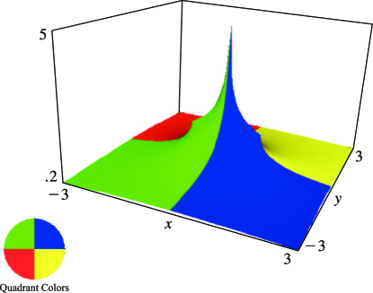
Figure 4.15.13: $\mathrm{arccsc}\left(x+\mathrm{i}y\right)$ (principal value). There is a branch cut along the real axis from $-1$ to $1$. Magnify 3D Help

…

12: 36.11 Leading-Order Asymptotics

… ►With real critical points (36.4.1) ordered so that … ►

Asymptotics along Symmetry Lines

… ►

36.11.5 $${\mathrm{\Psi }}_3\left(0,y,0\right)=\overline{{\mathrm{\Psi }}_3(0,-y,0)}=\exp \left(\frac{1}{4}\mathrm{i}\pi \right)\sqrt{\pi /y}\left(1-(\mathrm{i}/\sqrt{3})\exp \left(\frac{3}{2}\mathrm{i}{(2y/5)}^{5/3}\right)+o\left(1\right)\right),$$ $y\to +\mathrm{\infty }$.

ⓘ

Symbols:

${\mathrm{\Psi }}_K\left(𝐱\right)$: canonical integral function, $\pi$: the ratio of the circumference of a circle to its diameter, $\overline{z}$: complex conjugate, $\exp z$: exponential function, $\mathrm{i}$: imaginary unit, $o\left(x\right)$: order less than and $y$: real parameter

Permalink:

http://dlmf.nist.gov/36.11.E5

Encodings:

pMML, png, TeX

See also:

Annotations for §36.11, §36.11 and Ch.36

… ►

36.11.7 $${\mathrm{\Psi }}^{(\mathrm{E})}\left(0,0,z\right)=\frac{\pi }{z}\left(\mathrm{i}+\sqrt{3}\exp \left(\frac{4}{27}\mathrm{i}{z}^3\right)+o\left(1\right)\right),$$ $z\to \pm \mathrm{\infty }$,

ⓘ

Symbols:

$\pi$: the ratio of the circumference of a circle to its diameter, ${\mathrm{\Psi }}^{(\mathrm{E})}\left(𝐱\right)$: elliptic umbilic canonical integral function, $\exp z$: exponential function, $\mathrm{i}$: imaginary unit, $o\left(x\right)$: order less than and $z$: real parameter

Permalink:

http://dlmf.nist.gov/36.11.E7

Encodings:

pMML, png, TeX

See also:

Annotations for §36.11, §36.11 and Ch.36

►

36.11.8 $${\mathrm{\Psi }}^{(\mathrm{H})}\left(0,0,z\right)=\frac{2\pi }{z}\left(1-\frac{\mathrm{i}}{\sqrt{3}}\exp \left(\frac{1}{27}\mathrm{i}{z}^3\right)+o\left(1\right)\right),$$ $z\to \pm \mathrm{\infty }$.

ⓘ

Symbols:

$\pi$: the ratio of the circumference of a circle to its diameter, $\exp z$: exponential function, ${\mathrm{\Psi }}^{(\mathrm{H})}\left(𝐱\right)$: hyperbolic umbilic canonical integral function, $\mathrm{i}$: imaginary unit, $o\left(x\right)$: order less than and $z$: real parameter

Permalink:

http://dlmf.nist.gov/36.11.E8

Encodings:

pMML, png, TeX

See also:

Annotations for §36.11, §36.11 and Ch.36

13: 31.11 Expansions in Series of Hypergeometric Functions

… ►

31.11.3 $$\lambda +\mu =\gamma +\delta -1=\alpha +\beta -ϵ.$$

ⓘ

Defines:

$\lambda$ (locally) and $\mu$ (locally)

Symbols:

$\gamma$: real or complex parameter, $\delta$: real or complex parameter, $ϵ$: real or complex parameter, $\alpha$: real or complex parameter and $\beta$: real or complex parameter

Permalink:

http://dlmf.nist.gov/31.11.E3

Encodings:

pMML, png, TeX

See also:

Annotations for §31.11(ii), §31.11 and Ch.31

… ►

31.11.7 $$L_j=a(\lambda +j)(\mu -j)-q+\frac{(j+\alpha -\mu )(j+\beta -\mu )(j+\gamma -\mu )(j+\lambda )}{(2j+\lambda -\mu )(2j+\lambda -\mu +1)}+\frac{(j-\alpha +\lambda )(j-\beta +\lambda )(j-\gamma +\lambda )(j-\mu )}{(2j+\lambda -\mu )(2j+\lambda -\mu -1)},$$

ⓘ

Symbols:

$\gamma$: real or complex parameter, $j$: nonnegative integer, $a$: complex parameter, $q$: real or complex parameter, $\alpha$: real or complex parameter, $\beta$: real or complex parameter, $\lambda$ , $\mu$ and $L_j$: coefficients

Permalink:

http://dlmf.nist.gov/31.11.E7

Encodings:

pMML, png, TeX

See also:

Annotations for §31.11(ii), §31.11 and Ch.31

… ►

31.11.12 $$P_j^5=\frac{{\left(\alpha \right)}_j{\left(1-\gamma +\alpha \right)}_j}{{\left(1+\alpha -\beta +ϵ\right)}_{2j}}{z}^{-\alpha -j}{}_2{}^{}F_1^{}(\genfrac{}{}{0pt}{}{\alpha +j,1-\gamma +\alpha +j}{1+\alpha -\beta +ϵ+2j};\frac{1}{z}),$$

ⓘ

Symbols:

${}_2{}^{}F_1^{}(a,b;c;z)$: $=F(a,b;c;z)$ notation for Gauss’ hypergeometric function, ${\left(a\right)}_n$: Pochhammer’s symbol (or shifted factorial), $z$: complex variable, $\gamma$: real or complex parameter, $ϵ$: real or complex parameter, $j$: nonnegative integer, $\alpha$: real or complex parameter, $\beta$: real or complex parameter and $P_j^5$: first Kummer solution at $\mathrm{\infty }$ of generalized hypergeometric differential equation

Referenced by:

§31.11(iii), §31.11(iii), §31.11(iii), Erratum (V1.1.7) for Subsection 31.11(iii)

Permalink:

http://dlmf.nist.gov/31.11.E12

Encodings:

pMML, png, TeX

Notational Change (effective with 1.1.7):

We have rewritten the gamma functions in the prefactor more concisely using Pochhammer symbols.

See also:

Annotations for §31.11(iii), §31.11 and Ch.31

… ►Every Heun function (§31.4) can be represented by a series of Type I convergent in the whole plane cut along a line joining the two singularities of the Heun function. … ►The expansion (31.11.1) with (31.11.12) is convergent in the plane cut along the line joining the two singularities $z=0$ and $z=1$. …

14: 36.5 Stokes Sets

… ►where $j$ denotes a real critical point (36.4.1) or (36.4.2), and $\mu$ denotes a critical point with complex $t$ or $s,t$, connected with $j$ by a steepest-descent path (that is, a path where $\mathrm{\Re }\mathrm{\Phi }=\mathrm{constant}$) in complex $t$ or $(s,t)$ space. ►In the following subsections, only Stokes sets involving at least one real saddle are included unless stated otherwise. … ►The second sheet corresponds to $x>0$ and it intersects the bifurcation set (§36.4) smoothly along the line generated by $X=X_1=6.95643$, $\left|Y\right|=\left|Y_1\right|=6.81337$. … ►the intersection lines with the bifurcation set are generated by $|X|=X_2=0.45148$, $Y=Y_2=0.59693$. … ►The distribution of real and complex critical points in Figures 36.5.5 and 36.5.6 follows from consistency with Figure 36.5.1 and the fact that there are four real saddles in the inner regions. …

15: 10.20 Uniform Asymptotic Expansions for Large Order

… ►

§10.20(i) Real Variables

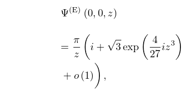
… ►As $\nu \to \mathrm{\infty }$ through positive real values … ►The function $\zeta =\zeta (z)$ given by (10.20.2) and (10.20.3) can be continued analytically to the $z$-plane cut along the negative real axis. … ►The curves $B{P}_1{E}_1$ and $B{P}_2{E}_2$ in the $z$-plane are the inverse maps of the line segments … ►As $\nu \to \mathrm{\infty }$ through positive real values the expansions (10.20.4)–(10.20.9) apply uniformly for $|\mathrm{ph}z|\le \pi -\delta$, the coefficients $A_k(\zeta )$, $B_k(\zeta )$, $C_k(\zeta )$, and $D_k(\zeta )$, being the analytic continuations of the functions defined in §10.20(i) when $\zeta$ is real. …

16: 30.13 Wave Equation in Prolate Spheroidal Coordinates

… ►The focal line is given by $\xi =1$, $-1\le \eta \le 1$, and the rays $\pm z\ge c$, $x=y=0$ are given by $\eta =\pm 1$, $\xi \ge 1$. … ►

30.13.3 $$h_{\xi }^2={\left(\frac{\partial x}{\partial \xi }\right)}^2+{\left(\frac{\partial y}{\partial \xi }\right)}^2+{\left(\frac{\partial z}{\partial \xi }\right)}^2=\frac{c^2({\xi }^2-{\eta }^2)}{{\xi }^2-1},$$

ⓘ

Symbols:

$\frac{\partial f}{\partial x}$: partial derivative of $f$ with respect to $x$ , $\partial x$: partial differential of $x$ , $z$: complex variable, $x$: real variable, $y$: real variable, $\xi$: prolate spheroidal coordinate, $\eta$: prolate spheroidal coordinate, $c$: positive constant and $h_{\xi },h_{\eta },h_{\varphi }$: metric coefficients

A&S Ref:

21.4.2

Permalink:

http://dlmf.nist.gov/30.13.E3

Encodings:

pMML, png, TeX

See also:

Annotations for §30.13(ii), §30.13 and Ch.30

… ►

30.13.11 $$\frac{d^2{w}_3}{{d\varphi }^2}+{\mu }^2{w}_3=0,$$

ⓘ

Symbols:

$\frac{df}{dx}$: derivative of $f$ with respect to $x$ , $\varphi$: prolate spheroidal coordinate, $w_j$: solution to DE and $\mu$: real parameter

Referenced by:

§30.14(iv)

Permalink:

http://dlmf.nist.gov/30.13.E11

Encodings:

pMML, png, TeX

See also:

Annotations for §30.13(iv), §30.13 and Ch.30

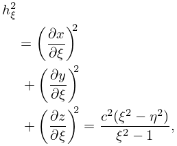
… ►Moreover, $w$ has to be bounded along the $z$-axis away from the focal line: this requires $w_2(\eta )$ to be bounded when . … ►If $b_2=0$, then this property holds outside the focal line. …

17: 1.18 Linear Second Order Differential Operators and Eigenfunction Expansions

… ►The space $X$ is now the full real line, $(-\mathrm{\infty },\mathrm{\infty })$. … ►This will be generalized, along with the choice of $X$, in §1.18(vii). … ►For this latter see Simon (1973), and Reinhardt (1982); wherein advantage is taken of the fact that although branch points are actual singularities of an analytic function, the location of the branch cuts are often at our disposal, as they are not singularities of the function, but simply arbitrary lines to keep a function single valued, and thus only singularities of a specific representation of that analytic function. … ►Suppose that $X$ is the whole real line in one dimension, and that $q(x)$, in (1.18.28) has (non-oscillatory) limits of $0$ at both $\pm \mathrm{\infty }$, and thus a continuous spectrum on $𝝈\ge 0$. …Surprisingly, if on any interval on the real line, even if positive elsewhere, as long as ${\int }_{X}q(x)dx\le 0$, see Simon (1976, Theorem 2.5), then there will be at least one eigenfunction with a negative eigenvalue, with corresponding $L^2\left(X\right)$ eigenfunction. …

18: 28.33 Physical Applications

… ►

28.33.1 $$\frac{{\partial }^{2}W}{{\partial x}^2}+\frac{{\partial }^{2}W}{{\partial y}^2}-\frac{\rho }{\tau }\frac{{\partial }^{2}W}{{\partial t}^2}=0,$$

ⓘ

Symbols:

$\frac{\partial f}{\partial x}$: partial derivative of $f$ with respect to $x$ , $\partial x$: partial differential of $x$ , $x$: real variable, $y$: real variable, $\rho$: mass, $\tau$: radial tension and $W(x,y,t)$: solution

Permalink:

http://dlmf.nist.gov/28.33.E1

Encodings:

pMML, png, TeX

See also:

Annotations for §28.33(ii), §28.33 and Ch.28

… ►As $\omega$ runs from $0$ to $+\mathrm{\infty }$, with $b$ and $f$ fixed, the point $(q,a)$ moves from $\mathrm{\infty }$ to $0$ along the ray $ℒ$ given by the part of the line $a=(2b/f)q$ that lies in the first quadrant of the $(q,a)$-plane. …