Whittaker equation

SearchAdvancedHelp

(0.003 seconds)

11—20 of 60 matching pages

11: 22.13 Derivatives and Differential Equations

§22.13 Derivatives and Differential Equations

… ►

§22.13(ii) First-Order Differential Equations

… ►

§22.13(iii) Second-Order Differential Equations

…

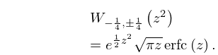
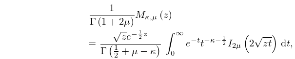
12: 13.18 Relations to Other Functions

… ►

13.18.7 $$W_{-\frac{1}{4},\pm \frac{1}{4}}\left(z^2\right)={\mathrm{e}}^{\frac{1}{2}{z}^2}\sqrt{\pi z}\mathrm{erfc}\left(z\right).$$

ⓘ

Symbols:

$W_{\kappa ,\mu }\left(z\right)$: Whittaker confluent hypergeometric function, $\pi$: the ratio of the circumference of a circle to its diameter, $\mathrm{erfc}z$: complementary error function, $\mathrm{e}$: base of natural logarithm and $z$: complex variable

Referenced by:

Erratum (V1.0.3) for Equation (13.18.7)

Permalink:

http://dlmf.nist.gov/13.18.E7

Encodings:

pMML, png, TeX

Clarification (effective with 1.0.3):

Originally the left-hand side was given correctly as $W_{-\frac{1}{4},-\frac{1}{4}}\left(z^2\right)$; the equation is true also for $W_{-\frac{1}{4},+\frac{1}{4}}\left(z^2\right)$.

See also:

Annotations for §13.18(ii), §13.18 and Ch.13

…

13: 31.8 Solutions via Quadratures

… ►For $𝐦=(m_0,0,0,0)$, these solutions reduce to Hermite’s solutions (Whittaker and Watson (1927, §23.7)) of the Lamé equation in its algebraic form. …

14: 13.29 Methods of Computation

… ►Similarly for the Whittaker functions. ►

§13.29(ii) Differential Equations

… ►For $M(a,b,z)$ and $M_{\kappa ,\mu }\left(z\right)$ this means that in the sector $|\mathrm{ph}z|\le \pi$ we may integrate along outward rays from the origin with initial values obtained from (13.2.2) and (13.14.2). ►For $U(a,b,z)$ and $W_{\kappa ,\mu }\left(z\right)$ we may integrate along outward rays from the origin in the sectors , with initial values obtained from connection formulas in §13.2(vii), §13.14(vii). … ►The integral representations (13.4.1) and (13.4.4) can be used to compute the Kummer functions, and (13.16.1) and (13.16.5) for the Whittaker functions. …

15: 18.39 Applications in the Physical Sciences

… ►These eigenfunctions are the orthonormal eigenfunctions of the time-independent Schrödinger equation … ►argument b) The Morse Oscillator …The corresponding eigenfunction transform is a generalization of the Kontorovich–Lebedev transform §10.43(v), see Faraut (1982, §IV). … ►The Schrödinger equation with potential … ►

Other Analytically Solved Schrödinger Equations

…

16: 5.9 Integral Representations

… ►

5.9.10_2 $$\mathrm{Ln}\mathrm{\Gamma }\left(z\right)=\left(z-\frac{1}{2}\right)\ln z-z+\frac{1}{2}\ln \left(2\pi \right)+{\int }_0^{\mathrm{\infty }}{\mathrm{e}}^{-zt}\left(\frac{1}{{\mathrm{e}}^t-1}-\frac{1}{t}+\frac{1}{2}\right)\frac{dt}{t},$$

ⓘ

Symbols:

$\mathrm{\Gamma }\left(z\right)$: gamma function, $\pi$: the ratio of the circumference of a circle to its diameter, $dx$: differential of $x$ , $\mathrm{e}$: base of natural logarithm, $\int$: integral, $\mathrm{Ln}z$: general logarithm function, $\ln z$: principal branch of logarithm function and $z$: complex variable

Source:

Whittaker and Watson (1927, §12.31)

Referenced by:

§5.9(i), Erratum (V1.1.7) for Additions

Permalink:

http://dlmf.nist.gov/5.9.E10_2

Encodings:

pMML, png, TeX

Addition (effective with 1.1.7):

This equation was added.

See also:

Annotations for §5.9(i), §5.9(i), §5.9 and Ch.5

…

17: Errata

… ►

18.34.1 $$y_n(x;a)={}_2{}^{}F_0^{}(\genfrac{}{}{0pt}{}{-n,n+a-1}{-};-\frac{x}{2})={\left(n+a-1\right)}_n{\left(\frac{x}{2}\right)}^n{}_1{}^{}F_1^{}(\genfrac{}{}{0pt}{}{-n}{-2n-a+2};\frac{2}{x})=n!{\left(-\frac{1}{2}x\right)}^n{L}_n^{(1-a-2n)}\left(2x^{-1}\right)={\left(\frac{1}{2}x\right)}^{1-\frac{1}{2}a}{\mathrm{e}}^{1/x}{W}_{1-\frac{1}{2}a,\frac{1}{2}(a-1)+n}\left(2x^{-1}\right)$$

This equation was updated to include the definition of Bessel polynomials in terms of Laguerre polynomials and the Whittaker confluent hypergeometric function.

… ►

28.8.5 $$V_m(\xi )\sim \frac{1}{2^{4}h}\left(-D_{m+2}\left(\xi \right)-m(m-1)D_{m-2}\left(\xi \right)\right)+\frac{1}{2^{10}{h}^2}\left(D_{m+6}\left(\xi \right)+(m^2-25m-36)D_{m+2}\left(\xi \right)-m(m-1)(m^2+27m-10)D_{m-2}\left(\xi \right)-6!\left(\genfrac{}{}{0.0pt}{}{m}{6}\right)D_{m-6}\left(\xi \right)\right)+\mathrm{\cdots }$$

Originally the $-$ in front of the $6!$ was given incorrectly as $+$.

Reported 2017-02-02 by Daniel Karlsson.

… ►

A sentence was added in §8.18(ii) to refer to Nemes and Olde Daalhuis (2016). Originally §8.11(iii) was applicable for real variables $a$ and $x=\lambda a$. It has been extended to allow for complex variables $a$ and $z=\lambda a$ (and we have replaced $x$ with $z$ in the subsection heading and in Equations (8.11.6) and (8.11.7)). Also, we have added two paragraphs after (8.11.9) to replace the original paragraph that appeared there. Furthermore, the interval of validity of (8.11.6) was increased from to the sector , and the interval of validity of (8.11.7) was increased from $\lambda >1$ to the sector $\lambda >1$, $|\mathrm{ph}a|\le \frac{3\pi }{2}-\delta$. A paragraph with reference to Nemes (2016) has been added in §8.11(v), and the sector of validity for (8.11.12) was increased from $|\mathrm{ph}z|\le \pi -\delta$ to $|\mathrm{ph}z|\le 2\pi -\delta$. Two new Subsections 13.6(vii), 13.18(vi), both entitled Coulomb Functions, were added to note the relationship of the Kummer and Whittaker functions to various forms of the Coulomb functions. A sentence was added in both §13.10(vi) and §13.23(v) noting that certain generalized orthogonality can be expressed in terms of Kummer functions.

… ►

13.18.7 $$W_{-\frac{1}{4},\pm \frac{1}{4}}\left(z^2\right)={\mathrm{e}}^{\frac{1}{2}{z}^2}\sqrt{\pi z}\mathrm{erfc}\left(z\right)$$

Originally the left-hand side was given correctly as $W_{-\frac{1}{4},-\frac{1}{4}}\left(z^2\right)$; the equation is true also for $W_{-\frac{1}{4},+\frac{1}{4}}\left(z^2\right)$.

…

18: 20.13 Physical Applications

… ►The functions ${\theta }_j\left(z\right|\tau )$, $j=1,2,3,4$, provide periodic solutions of the partial differential equation …with $\kappa =-\mathrm{i}\pi /4$. ►For $\tau =\mathrm{i}t$, with $\alpha ,t,z$ real, (20.13.1) takes the form of a real-time $t$ diffusion equation …Theta-function solutions to the heat diffusion equation with simple boundary conditions are discussed in Lawden (1989, pp. 1–3), and with more general boundary conditions in Körner (1989, pp. 274–281). … ►This allows analytic time propagation of quantum wave-packets in a box, or on a ring, as closed-form solutions of the time-dependent Schrödinger equation.

19: 13.16 Integral Representations

… ►

13.16.4 $$\frac{1}{\mathrm{\Gamma }\left(1+2\mu \right)}{M}_{\kappa ,\mu }\left(z\right)=\frac{\sqrt{z}{\mathrm{e}}^{-\frac{1}{2}z}}{\mathrm{\Gamma }\left(\frac{1}{2}+\mu -\kappa \right)}{\int }_0^{\mathrm{\infty }}{\mathrm{e}}^{-t}{t}^{-\kappa -\frac{1}{2}}{I}_{2\mu }\left(2\sqrt{zt}\right)dt,$$ .

ⓘ

Symbols:

$\mathrm{\Gamma }\left(z\right)$: gamma function, $M_{\kappa ,\mu }\left(z\right)$: Whittaker confluent hypergeometric function, $dx$: differential of $x$ , $\mathrm{e}$: base of natural logarithm, $\int$: integral, $I_{\nu }\left(z\right)$: modified Bessel function of the first kind, $\mathrm{\Re }$: real part and $z$: complex variable

Referenced by:

Erratum (V1.0.5) for Equation (13.16.4)

Permalink:

http://dlmf.nist.gov/13.16.E4

Encodings:

pMML, png, TeX

Errata (effective with 1.0.5):

Originally the condition for the validity of this equation was stated incorrectly as $\mathrm{\Re }(\kappa -\mu )-\frac{1}{2}>0$. The correct condition is .

See also:

Annotations for §13.16(i), §13.16 and Ch.13

…

20: Bibliography O

… ►

On the asymptotic solution of second-order differential equations having an irregular singularity of rank one, with an application to Whittaker functions. J. Soc. Indust. Appl. Math. Ser. B Numer. Anal. 2 (2), pp. 225–243.

ⓘ

External Links:

Document, MathReview (T. E. Hull), ZentralBlatt

Referenced by:

§13.19, §13.7(ii).

Encodings:

BibTeX

…